Practice/Exercise: Spatial Analysis Vector Data - Motorway
OpenSchoolMaps.ch — Free learning materials for free geodata and maps
Impact assessment of a motorway construction with QGIS 3
General information
The assessment of impairments of legally protected biotope types by traffic structures is a typical task of landscape planning. The task is based on the construction of the A44 through the German Lichtenau plateau without using the original data.
-
Effects of a motorway section on habitat types
-
Introduction to geodata processing
-
Working with buffers and intersections
This task is mainly based on Task 6 of the course “Introduction into GIS and digital cartography” by Claas Leiner, Uni Kassel, 2010.
Goals and specifications
The goal of this exercise is to assess the impact of motorway construction on habitat types Fauna-Flora-Habitat (FFH for short, a European legislative directive, see Wikipedia) and legally protected biotope types.
The working data are polygon vector data (layer “environment” in geopackage
autobahn_inputs.gpkg) with the results of a biotope type and usage mapping,
lines vector data (layer “autobahn_central line” in geopackage
autobahn_inputs.gpkg) with the central line of a fictitious motorway
route and the topographic map 1:25'000 (Tk25) (file heli.tif) as background.
In the functional data table of "environment", pieces of usage (impacts) that are to be assigned to a habitat type (ffh_typ_nr) are marked (ffh_typ_text). Likewise, specially protected biotope types according to federal law (abbreviated to BNatSchG) (field “geschuetzt_biotop”) and other types of species-rich grassland (“bedeutend_gruenland_typ”) are labelled.
You should determine the size of the valuable area from the point of view of species and biotope conservation that is completely destroyed or impaired by motorway construction. To answer this question, you can use the “buffer tool” to identify degradation zones at different distances from the central line, which are further intersected with biotope type mapping to identify degraded and unimpaired areas.
Finally, the results could be entered in a table as an area balance (optional).
-
QGIS (tested with QGIS 3.4)
-
Data:
-
autobahn_inputs.gpkg -
heli.tif
-
Tasks
Preparation: Creating the project file and loading the input data
-
Open QGIS and make sure that no existing project is open. (So only either a new, still empty and unsaved project or none at all.)
-
Load
autobahn_inputs.gpkgwith both vector layers included. -
If no project was open yet, a (not yet saved) one has been created automatically. Make sure that in the project settings the coordinate reference system (CRS) is set to the German DHDN Gauss-Krüger Zone 3 (EPSG:31467). (This should be the case automatically after loading the layers.)
-
Open the project settings via the menu , give the project the title "Motorway and habitat types" under the tab “General” and save it under the name
Autobahn_Lebensraumtypen.qgzorAutobahn_Lebensraumtypen.qgs.
Task 1: Presentation of land use
-
Classify layers "environment" using the attribute bfn_biotop_text to get an overview of the biotope types. A coarser representation of land use can be achieved by classifying land use according to the "use" field. Work out a meaningful representation using colors and textures. Present your classification as a map.
-
Create a map layout and export it as
biotoptypen.pdf. If you are using textures, you should check the "Print as raster" box on the “General > Print quality” tab in the print composition before exporting.
Task 2: Displaying the motorway central line and creating the buffer zones
Let’s now turn to the motorway central line in Layer autobahn_zentrallinie.
-
Make the line clearly visible.
-
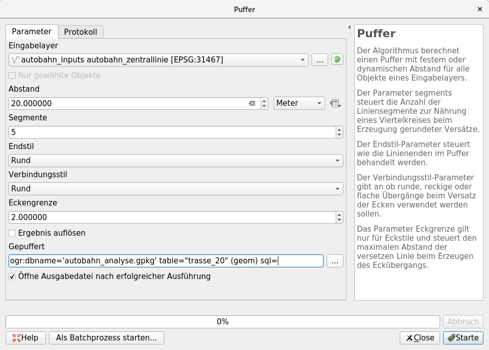
The motorway body measures 40m in total. For a two-dimensional representation you have to create a buffer polygon with a distance of 20 m from the center line on both sides.
You can do this via the menu . The "Input layer" is the "Motorway central line", the "distance" is 20 meters.
-
We want to record the result of this process in a file. To save it as a layer in a new file, click the … button next to the layer name field and choose Save as Geopackage…. Name the new file
autobahn_analyse.gpkgand the new layer route_20. -
Execute the processing with the button Start.
Now you see the highway body in your study area.
-
Even if the layer in the new file is now called
trasse_20.gpkg, it may have been labeled "buffered" in QGIS. Rename it to “route_20” if necessary. This is possible via the layer properties, which you can access e.g. via the context menu of the layer entry in the layer panel. -
The impairments of the motorway extend beyond the motorway route. Therefore you have to create more buffer zones.
Create two more "buffers" starting from the route you just created:
-
One with a distance of 100 m as temporary layer route_20_buffer_100
-
A 300 m apart temporary layer route_20_buffer_300.
route_20_buffer_100 identifies the areas immediately adjacent to the motorway in which major impairments due to exhaust fumes, noise and waste water are to be expected. The area of route_20_buffer_300 includes the further intervention area up to a distance of 300 m from the motorway.
-
-
Also here it is possible that the temporary files created in the background for the layers are called as required, but the layers are listed as "buffered" in QGIS. Rename them accordingly.
Task 3: Create Ring Zones Excluding the Buffer Zones
All buffer polygons created cover the entire area between your outer borders. The large buffer areas cover the small zones. However, we need polygons in the form of adjoining zones that do not overlap. In order to achieve this goal, we use the tool “difference” for testing purposes. After the following intersection processes you have the body of the motorway as well as two enclosing and adjoining shells around the motorway.
Creation of the external zone (from 100 m to 300 m distance from the motorway):
-
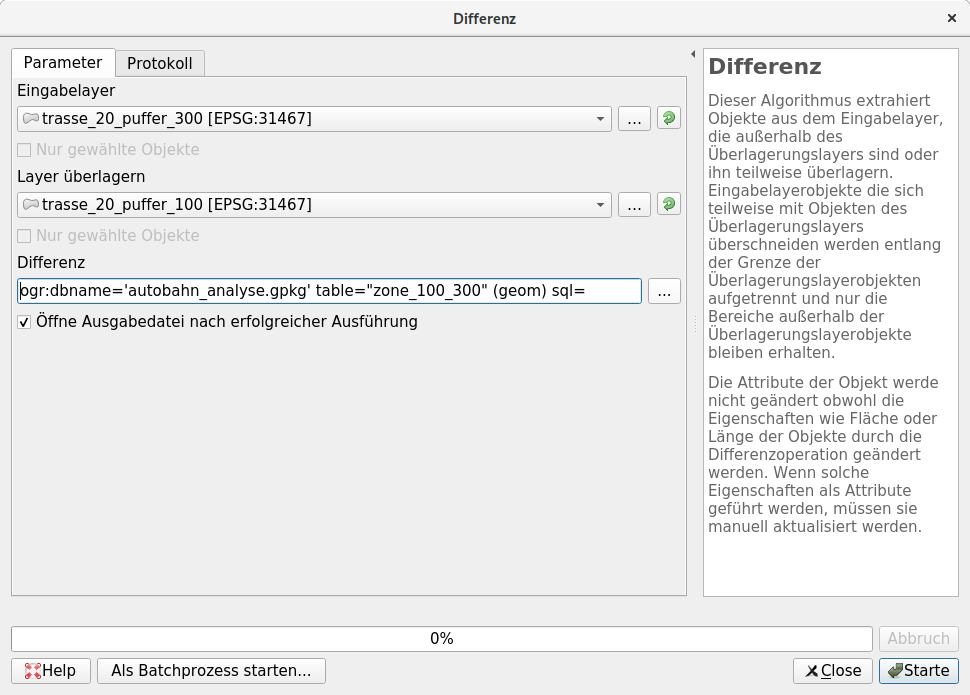
The area of the buffer route_20_buffer_100 must be cut out of the buffer route_20_buffer_300 in order to demarcate the external impairment zone.
This can be achieved with the menu option .
-
“Input layer” = route_20_buffer_300
-
“Layer overlay” = route_20_buffer_100
-
-
Save the result in the existing file
autobahn_analyse.gpkgas a new layer zone_100_300. -
Also here it is possible that QGIS saves the layer under the correct name, but integrates it into the project itself as "difference". Rename it to zone_100_300 if necessary.
Creation of the internal zone (from the route to 100 m from the motorway).
-
The area of the buffer route_20 must be cut out of the buffer route_20_buffer_100 in order to delimit the inner impairment zone. Save it as Layer zone_100 also in
analyse.gpkgand rename the layer to QGIS if necessary.-
“Input layer” = route_20_buffer_100
-
“Layer overlay” = route_20
-
The following layers are now important:
-
The two layers with the input data
-
The actual 40 metre wide route: route_20
-
The zone from the route to a distance of 100 m: zone_100
-
The zone at a distance of 100 m up to 300 m from the route: zone_100_300
If everything went fine, you can hide or delete the two temporary layers for a better overview:
-
route_20_buffer_100
-
route_20_buffer_300
Task 4: Merge the three zones into one layer
With the Merge tool, any number of geometries can be merged into one layer in one step.
-
Select Merge vector layer… from the menu
-
Choose as the input layer:
-
route_20
-
zone_100
-
zone_100_300
-
-
Save the result in
autobahn_analyse.gpkgas layer “zones”. -
Also here it can be that QGIS integrates the new layer under a generic name (here: "merged"). Rename it to
zonesif necessary.
Task 5: Edit the attribute table of the vector file alle_zonen.shp.
The new layer does not yet have meaningful attribute values for the individual impairment zones. You must assign an attribute value to the zones so that you can determine the area of differently rated biotope types in the impairment zones. Edit the attribute table in the layer properties
-
Open the context menu of the layer "zones" and choose Properties….
-
In the layer properties window, select the "source fields" tab.
-
Activate the editing mode (button with the pen)
-
Delete all fields except “layer” and “fid”.
-
Rename the field “layer” to “zone”.
-
Close the Layer Properties window with OK.
-
Open the context menu of the layer "zones" and choose Open attribute table.
-
Change the values in the
zonecolumn as follows:-
route_20 → Route
-
zone_100 → Inside
-
zone_100_300 → Outside
-
-
You can then cut off the excess end curves of the buffers with the drawing tool (the cutting line can be completed with a right click), select these remaining areas via and then delete the remaining areas with the function .
-
Save the layer (menu ) and classify the zones. Use hatching or point density grids to avoid completely covering the underlying planes.
Task 6: Query of all areas of outstanding nature conservation expertise
Now all areas from the environment layer that are important for nature conservation are to be queried. These are habitat types in annex 1 of the Habitats Directive (ffh_typ_nr), specially protected biotope types in accordance with the Federal Nature Conservation Act (BNatSchG) (protected_biotope) and other biotope types of species-rich grassland (significant_green_land_type).
Proceed as follows:
-
Select the layer “environment” in the layer panel.
-
Open the attribute table () to get an overview. (After that you can close the attribute table again.)
-
Open the query editor via the menu option .
-
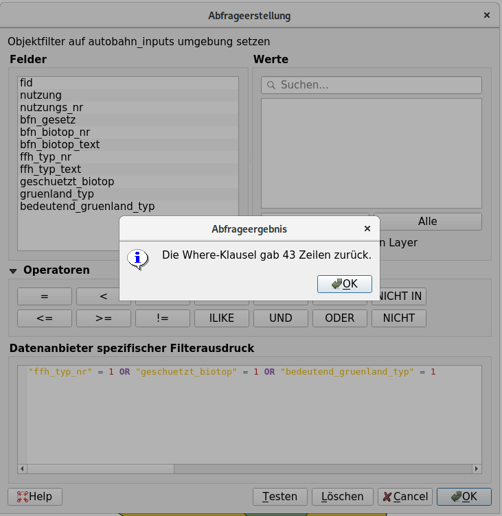
Create a query using the query editor buttons to select all areas that are either FFH habitats (
ffh_typ_nr = 1), protected biotopes (OR protected_biotop = 1), or other significant grassland types (OR significant_greenland_typ = 1).Note: In the relevant columns of the attribute table, the value
1means “applies` to”.Your SQL command must look like this:
ffh_typ_nr = 1 OR geschuetzt_biotop = 1 OR bedeutend_gruenland_typ = 1 -
Test the query.
The selection should contain 43 polygons.
-
Confirm with OK. This applies the filter to the layer and closes the query creation window. Now you can see all areas that are valuable from the point of view of biotope and species conservation.
-
Save the filtered layer(s) via in the geopackage
autobahn_analyse.gpkgas layer “valuable”. After that you can delete the filter on layer “environment” again.
Task 7: Intersection between valuable areas and impairment zones
The next step is to identify those areas of nature conservation value that are located in the three impaired zones. You’re using the “intersection” tool to intersect the layers valuable and zones with each other. The resulting layer contains only areas which are valuable for nature conservation and which are destroyed or impaired at the same time by motorway construction.
-
With the menu option you intersect both layers.
-
“Input Layer”: zones
-
“Layer overlay”: valuable
-
Target layer: Untitled Temporary Layer
-
-
A click on Start leads to the following error message:
Object (24) has invalid geometry. Please correct these errors or change the processing setting to "Ignore invalid input objects".
Execution failed after 0.01 seconds
Open the QGIS options via menu and change under tab “Processing” > section “General” the corresponding setting “Suspend invalid object filtering” from “Stop algorithm execution on invalid geometry” to “Ignore invalid geometry objects.”.
-
Now repeat the blending operation. Now it should succeed. The error message comes anyway, but with “finished” instead of “failed”.
-
The resulting layer has probably been included in QGIS under the name “intersection”. Rename it “intersect_valueful”.
-
Open the attribute table of the new layer. The values of the “fid”-column of the 2nd input layer (“valueful”) can be found in the column “fid_2” of the new layer. The “fid”-column of the 1st input layer (zones) is shown in the result as “fid” in “intersect_valueful” but as “fid”, which is problematic, because QGIS takes this column name as PK of e.g. GeoPackage layers by default, but the values are now anything but UNIQUE due to the intersection.
-
Rename the “fid”-column from “intersect_valueful” to “fid_zone” and end the editing mode.
-
Via its context menu you can now make layer “intersect_valueful” permanent. Save it as “intersect_valueful” in
autobahn_analyse.gpkg. Make sure that the name specified in the "FID" field does not correspond to an existing column. -
Now you can add “intersect_valueful” to the attribute table of the layer. (Menu ) click on the “Field Calculator” in the upper right corner. This allows you to create a new field based on an “expression”. Use the following expression to use QGIS to calculate the area of our polygon, which is then divided by 100 to convert the square meters to ares. The result is ultimately rounded to 1 significant digit after the decimal point. Expression: round($area / 100, 1)
-
Set “area” as “output field names” and select the “output field types” “decimal number (real)”. Confirm with OK and check if a column with the name “area” has been created.
-
Now in the column “area” you can find the exact areas of the polygons in ares.
-
Save the new column by deactivating the edit mode for the intersect_value layer.
Task 8: Classify vector files and create maps
Afterwards you should present your newly created geometries as meaningful maps. You should present the valuable biotope types in the impairment zones or the conflict zones as a map.
-
Classify Layer intersect_valueful by attribute ffh_typ_text (click on Classify).
-
Delete the empty value.
-
The layer now displays all areas within the affected zones where FFH-relevant biotope types are located.
-
Filter Layer intersect_valueful with the help of the query editor with the query ffh_typ_nr = 0.
-
Save the selection via under the layer name “intersect_valueful_without_ffh” in
autobahn_analyse.gpkg. -
Load the new layer and classify it by bfn_biotop_text
-
Delete the empty value and you get three classes of valuable non-FFFH biotopes.
-
Load the enclosed raster file
heli.tifand move it to the bottom of the table of contents. Then adjust the global transparency in the layer properties ofheli.tifso that the raster layer can serve as a weakly visible background. -
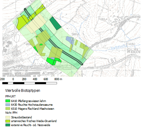
Now you can create a map which shows the valuable biotope types affected by the motorway construction and additionally highlights the ffh_typ_nr.
-
Create a map layout and export it as PDF. (Before doing this, activate “Print as Raster” under General)
-
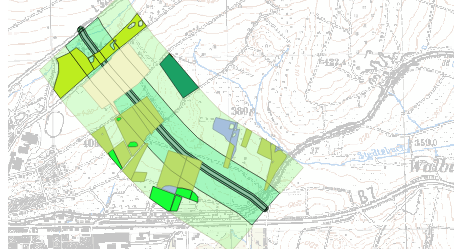
You can see an example of a possible map display on the following page. But you don’t have to create a layout with two cards. It is enough if you decide on a content statement and visualize it in a meaningful map layout.
Closure
The following files must now be present:
-
The simple biotope type map.
-
A finished map layout in PDF format, which represents either the valuable biotope types in the area of impairment or the conflict zones from the point of view of biotope and species protection.
Open questions? Please contact the QGIS-Community!
![]() Freely usable under CC0 1.0
Freely usable under CC0 1.0