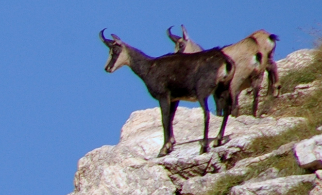
Practice/Exercise: Spatial Analysis Raster Data - Where The Chamois Live
OpenSchoolMaps.ch — Free learning materials for free geodata and maps
A multi-criteria raster analysis with QGIS 3
General information
Do you know where the chamois potentially live? A multi-criteria raster analysis with a GIS provides the answer. This exercise was originally written by Andreas Lienhard, Canton Zurich (many thanks!), and was then further developed.
-
Expenditure of time: This exercise takes at least 30 minutes if you already know something about QGIS.
-
Requirements: QGIS 3 (this exercise was created with QGIS version 3.6 and tested with QGIS 3.4 LTS).
-
Tags: GIS, Raster, Grid, Multi-criteria analysis, Raster algebra, QGIS.
Goals and specifications
The goal of this exercise is to use multi-criteria GIS analysis to find out where chamois potentially have their habitat. We make the following assumptions (criteria) for this purpose:
-
Chamois stay above 1500 m above sea level. We are also looking for chamois in spring, i.e. there is still a lot of snow starting at 2500 m.
-
Chamois are mainly found on steep slopes (slope >20%).
-
Chamois prefer warm, early leveled slopes, i.e. southern slopes.
-
Chamois use alpine pastures, because in spring there are no cattle on the alp.
The following two raster/grid data sets are available for the analysis (further information on the ASCII grid format can be found here http://giswiki.hsr.ch/Grid ):
-
Elevation model “DHM-Rimini” (originally from Swisstopo) in ArcInfo ASCII grid format, file
dhm_rimini.txt. (Elevation model: Digital Height Model, DHM) -
Statistical data “area statistics 85” (originally from BfS) in ArcInfo ASCII grid format, file
as85.txt. Contains soil cover species such as wad, meadows and pastures.
Preparations
After the specifications have been clarified, we can begin with the analysis of the potential chamois habitats. This is the schedule:
-
First the elevation model and the area statistics are loaded into QGIS.
-
With the elevation model, a terrain shading map is created in advance as a pure background.
-
With the elevation model, an inclination map and a terrain alignment map are calculated and saved as intermediate results.
-
Then partial results are calculated and saved according to the four criteria:
-
Starting from the elevation model, the corresponding elevation areas are filtered.
-
The steep slopes are filtered on the basis of the slope map.
-
Starting from the orientation map, the southern slopes are filtered.
-
Based on the area statistics, the alpine pastures are filtered.
-
-
Finally, the last four intermediate results are intersected (spatial overlay, intersection) and the result is visualized.
Now start QGIS - or open a new QGIS project - and change the project’s coordinate reference system to the old Swiss coordinate reference system EPSG:21781.
Import
To load the two input files as85.txt and dhm_rimini.txt
you can either drag and drop them into the QGIS or open the
menu .
There select Add Rasterlayer…
and specify the appropriate files.
Select as coordinate reference system EPSG:21781.
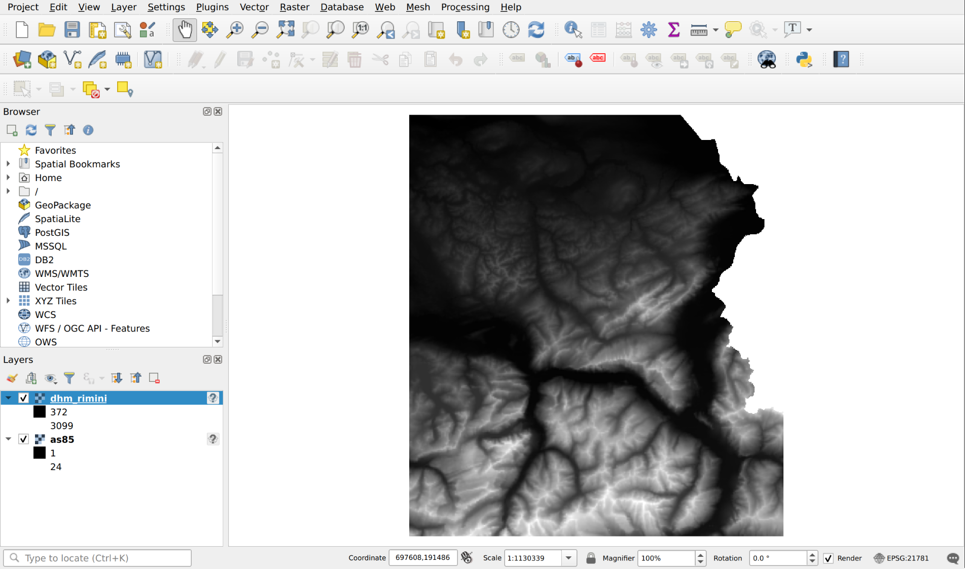
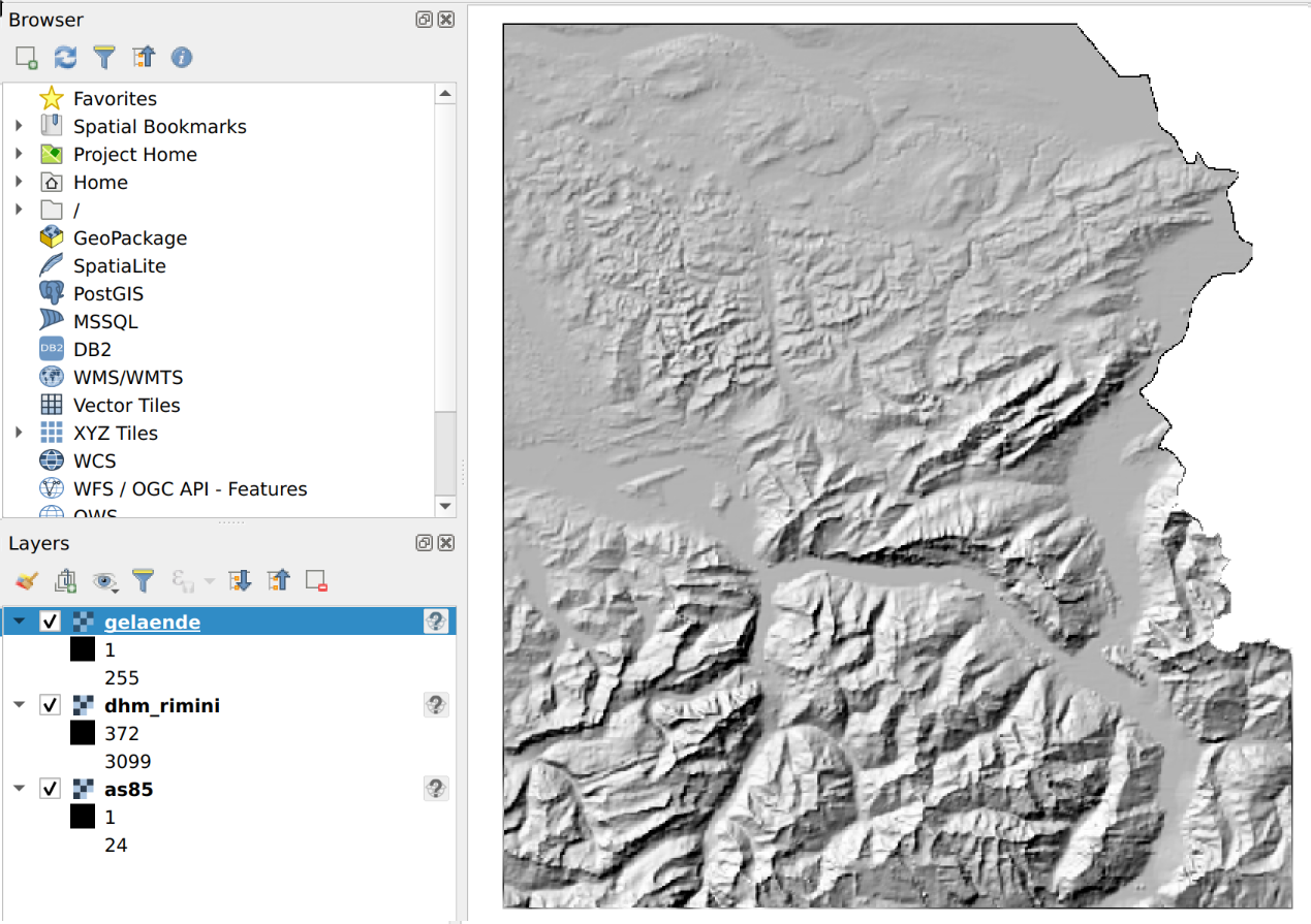
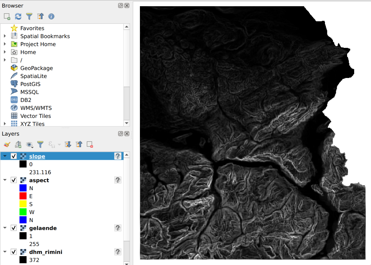
Check that the layer “dhm_rimini” is visible at the top of the layer manager, otherwise simply pull up the layer in the layer manager. If the layer is black, you can customize it by going to Layer Properties and changing "Contrast Enhancement" from "Cut to MinMax" to "Stretch to MinMax" (there are some more display options). Now you should see what is shown below.
Terrain shading map
This step is not yet part of the evaluation but rather serves for visualization and orientation on the map. The menu Raster allows you to edit and change the raster layers in QGIS. New layers are usually created and displayed in the QGIS project.
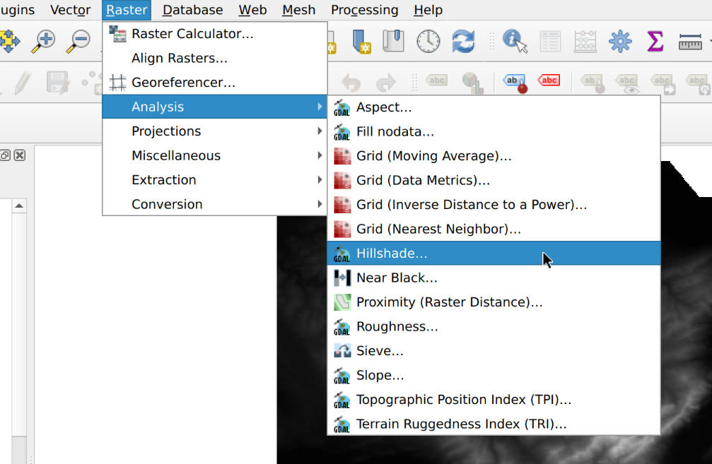
To create a terrain shading map from an elevation model, select menu (see figure below).
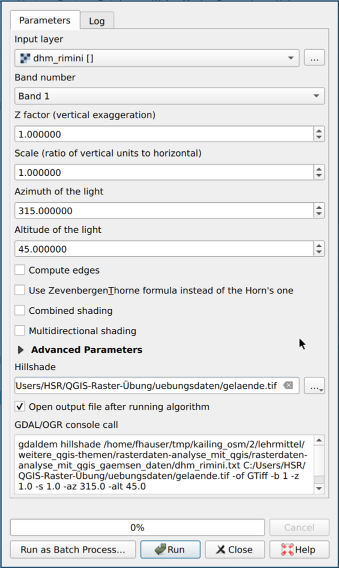
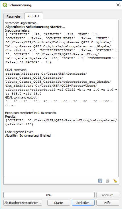
As input file you choose the layer “dhm_rimini”.
Click on "shading" (output file) right on …,
you open a new exercise data folder e.g. chamois
and enter the name terrain.tif
(the extension tif stands for TIFF or GeoTIFF).
After a click on Start the dialog window automatically changes to the tab with the execution protocol. You can then close the "Shading" window with the protocol. After that you should get about the following result with the terrain shading:
At this point also save the whole QGIS project in
the folder chamois with the name chamois.qgz.
Now we come in the next chapter to the first evaluation with the partial result "terrain alignment".
Terrain orientation map
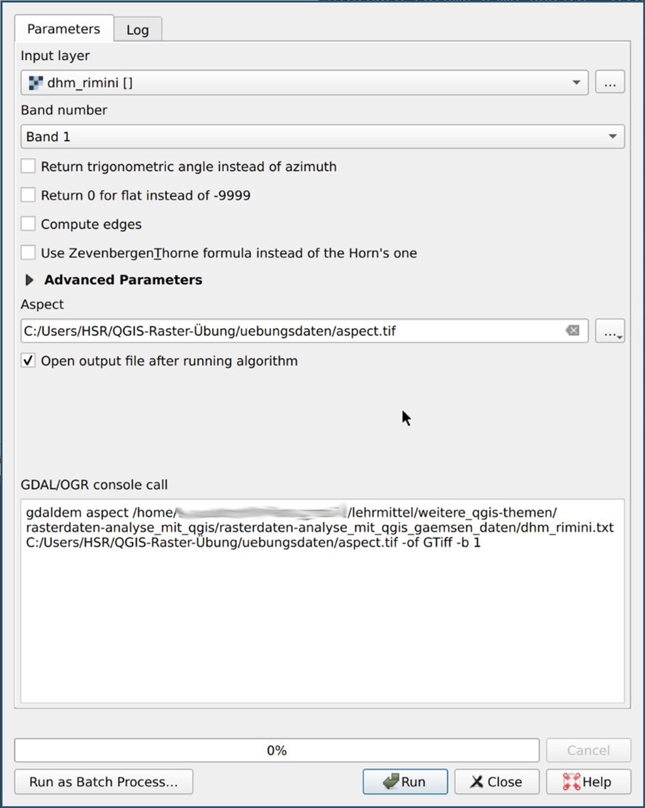
The terrain orientation map shows the aspect of the terrain in relation to the north. It is created with an elevation model as source via () (see figure above).
As input layer you choose “dhm_rimini” again.
Vote "Perspective" (output file), the exercise
data folder (gaemse) and the file name
aspect.tif: see figure above.
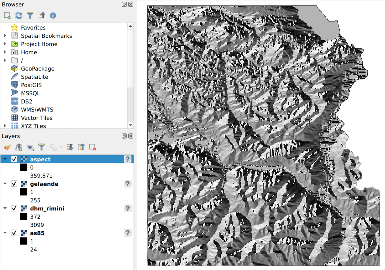
If everything went right, you should see something like this (may vary):
But now we want to improve this representation of the terrain alignment map a little bit. To change the style of a layer, right-click or double-click on the layer name and its properties.
In the “Symbolisation” in the first entry “Channel display”, select the display type “Singleband pseudocolor”. Only “Channel 1 (grey)” can be selected as the channel. Now you can set “Min” to 0 and “Max” and to 360, “Interpolation” to “Linear”, as "gradient" choose any one so that the automatic classification works (which gradient doesn’t matter as we will assign the colors manually), set the mode to "Equal Interval" and the number of classes to 5.
An orientation map contains as value an angle (in degrees °), which represents the orientation of the terrain. We want to assign different colors to the four main directions (N, E, S, W). The result of the operation used corresponds to 0° north (N). Values close to 0° therefore indicate a north slope. But also values close to 360° represent northern slopes. Therefore, five instead of only four classes were used. Therefore assign the same color to the first and last class, e.g. blue. The angle in the result is to be understood clockwise, i.e. 90° is East. Assign different, easily distinguishable colors to the remaining three classes, e.g. red, yellow, green.
If you want, you can give the classes a meaningful "label", e.g. N, E, S, W (and again N).
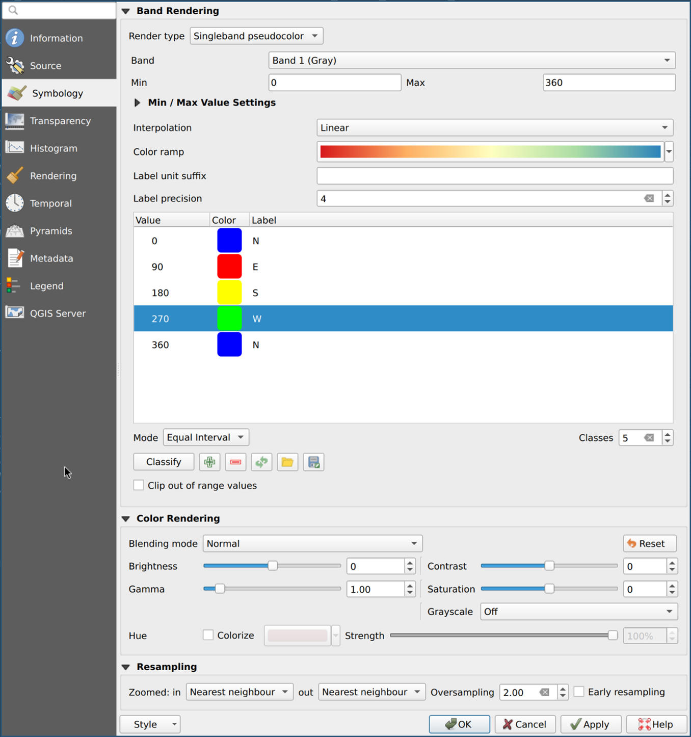
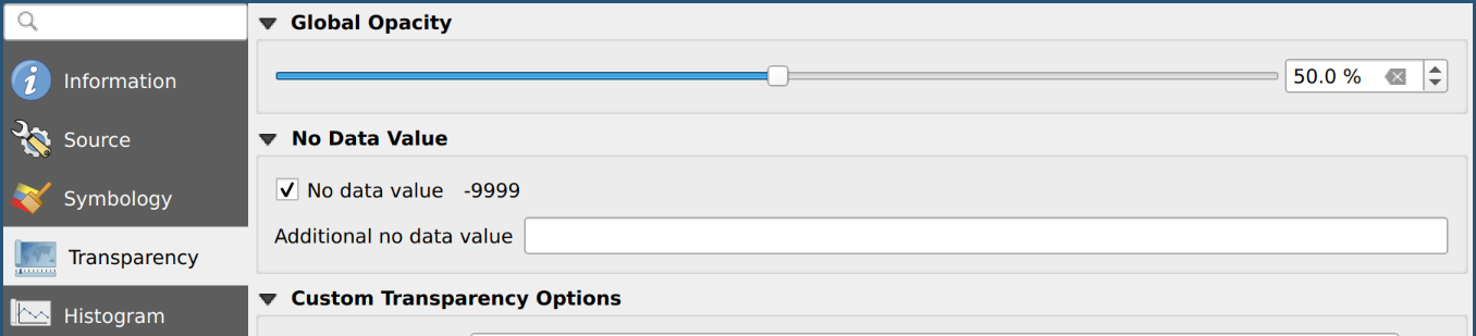
When you have made all the settings, go to the “Transparency” tab (below tab “Symbolisation”). Here we set the global transparency to e.g. 50% so that you can still see the shading under the coloured alignment map.
Then click on Ok (the dialog closes).
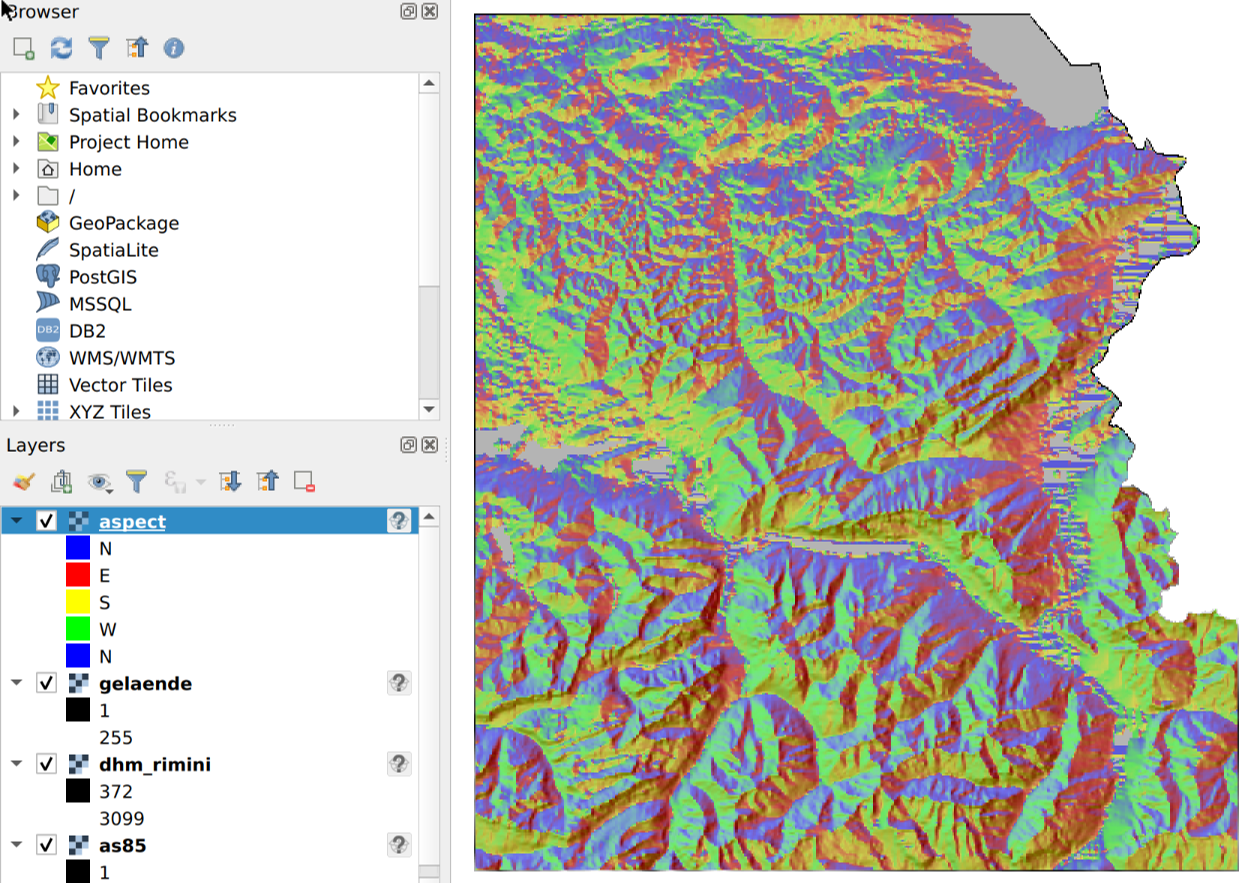
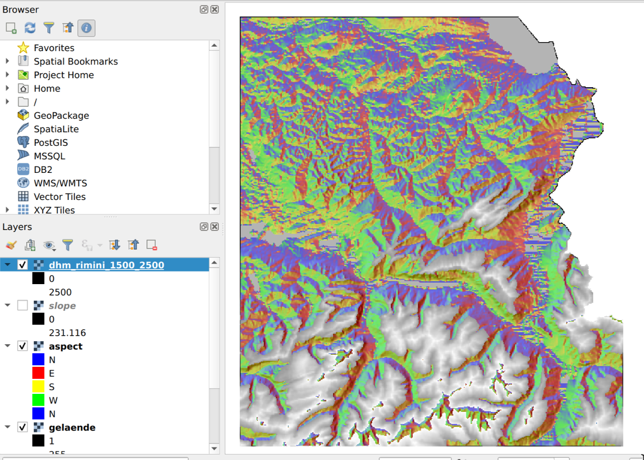
The result should look like the one shown below. If you’ve set other colors, it’s no big deal. The main thing is that the cardinal directions are now visualized by different colors.
Slope map
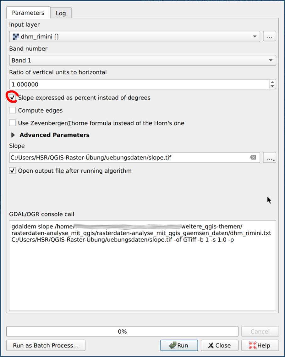
With the function “slope” (menu )
you can display the slope of a terrain coded as raster/grid.
For this exercise we want to express the gradient
in percent instead of degrees (see below).
As input file, select the layer “dhm_rimini” again
and enter the output file slope.tif in the exercise data folder.
Then Start.
The result looks like this (for "Contrast enhancement" on "Stretches on MinMax"):
Filter by criteria
You have now prepared the data so that we can apply the criteria. Just a reminder: We are looking for those areas that meet the following criteria:
-
Areas higher than 1500 m above sea level and lower than 2500 m above sea level.
-
Areas steeper than 20%.
-
South slope areas, i.e. areas with a south-east to south-west orientation.
-
Areas with the use of meadow and arable land, home pastures, spring pastures (Ger. "Maiensässe"), hay alps, mountain pastures, alpine pastures.
In order to meet these requirements, we now calculate four additional layers from the prepared data. A blend of these will show us where chamois could be. Cutting and filtering is done with the "raster algebra" and in QGIS with the raster calculator.
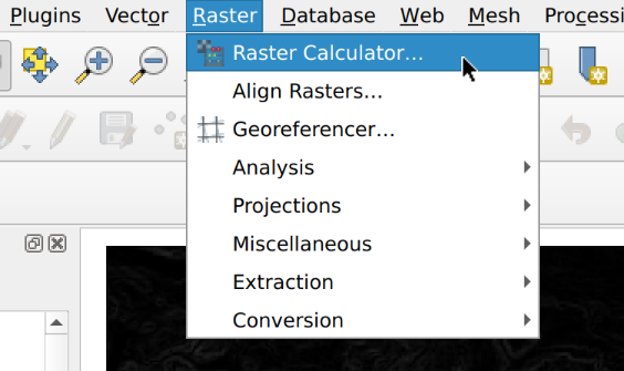
Let’s start with the first criterion: The heights of the terrain are stored in the layer “dhm_rimini”. Now we will calculate a new layer which contains only those grid cells which are between 1500 and 2500 m above sea level. For this you have to open the raster calculator via Raster.
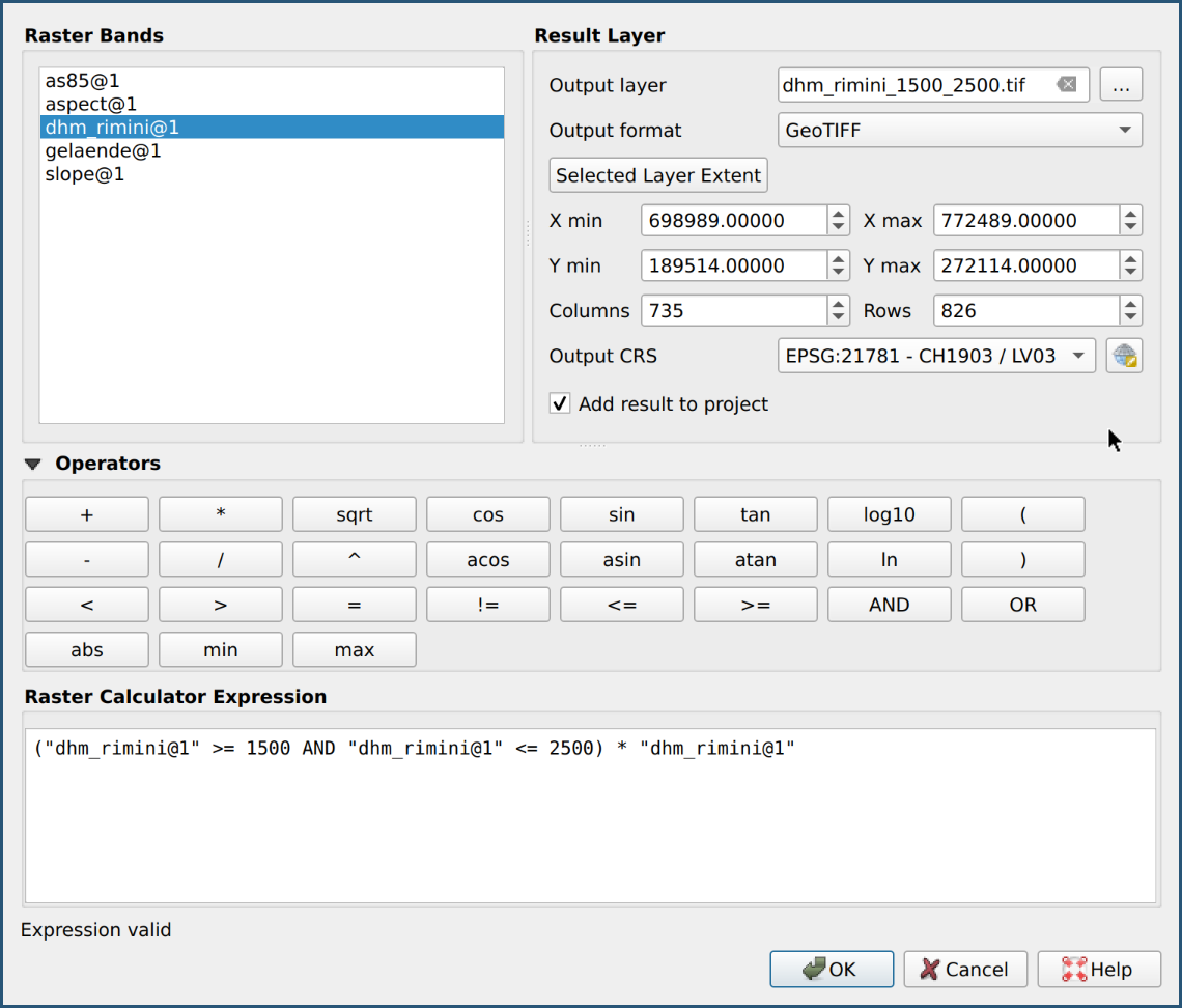
In the raster calculator you have to enter the output layer in the upper right corner.
Select the exercise data folder and name the output file dhm_rimini_1500_2500.tif.
On the left side of the dialog are the available layers
with their "raster channels" (here always “@1”).
For this first calculation we choose “dhm_rimini@1”.
Double-click it to add it to the raster calculator expression in quotation marks.
But the expression is not ready yet.
We would like to filter by values between 1500 and 2500.
For this we select the operators “larger-equal”/“smaller-equal”
(>= and <=), which we associate with AND and bracket.
Thus those values which lie in between get a 1.
But from these we would like to keep the original value.
We multiply the bracketed expression by the original value itself
(this is ingenious ☺, because the bracketed Boolean expression
is obviously interpreted as number 1/0 instead of true/false).
You can either type the expression directly or compile
it by clicking on the operator buttons in the "Operators" area.
Start the raster calculator with OK.
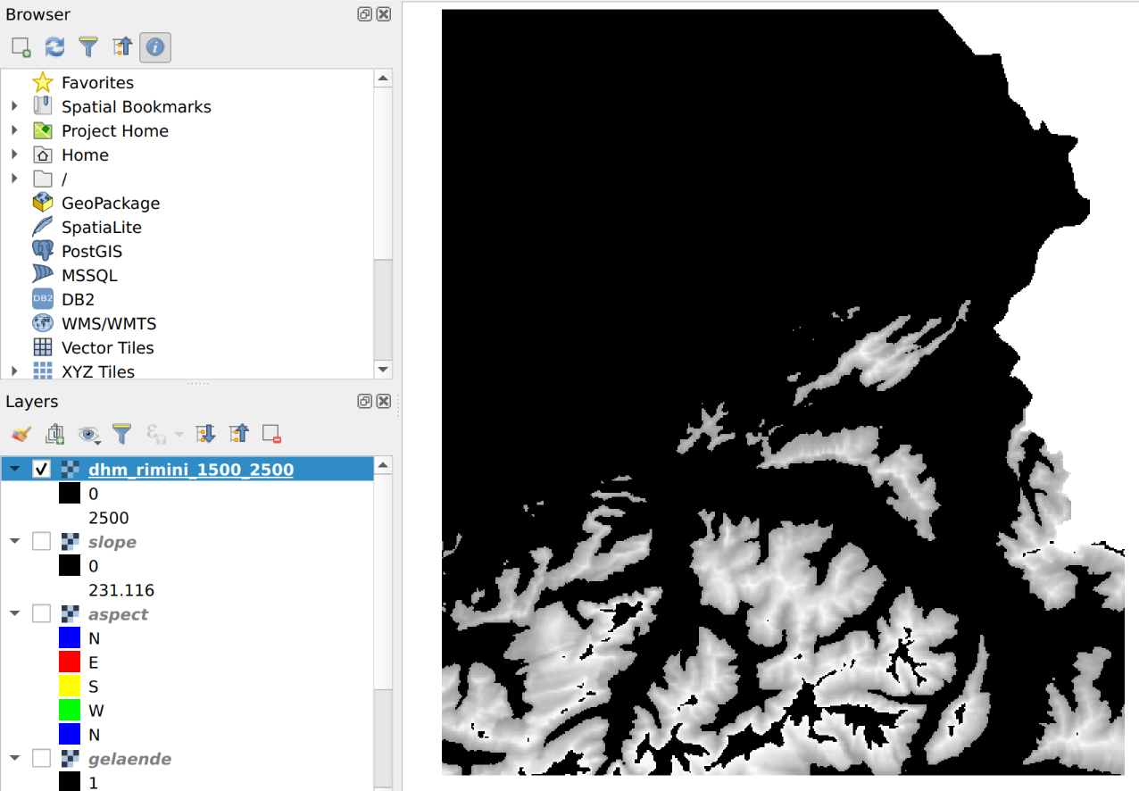
We can now check whether all the desired points have retained their value by clicking on “query objects” (the “i”-icon) and click with the mouse into the window: For black raster cells (pixels) the value 0 is displayed and for grey cells a value between 1500 m. a.s.l. and 2500 m. a.s.l. is displayed.
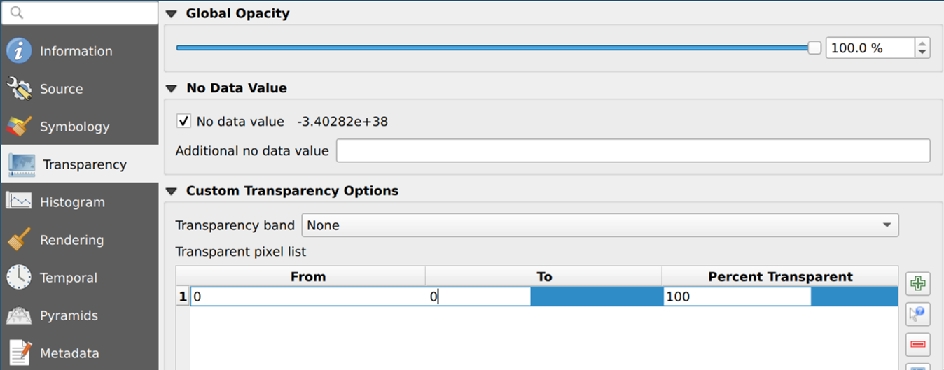
In order to filter out the 0 values from the view, we can assign them a transparency. In the Layer Properties > “Transparency” and “User defined transparency setting” click on + and set both values “From” and “To” to 0. Then click on Apply.
Now switch off the visibility of the layer “Inclination” in the Layer Manager.
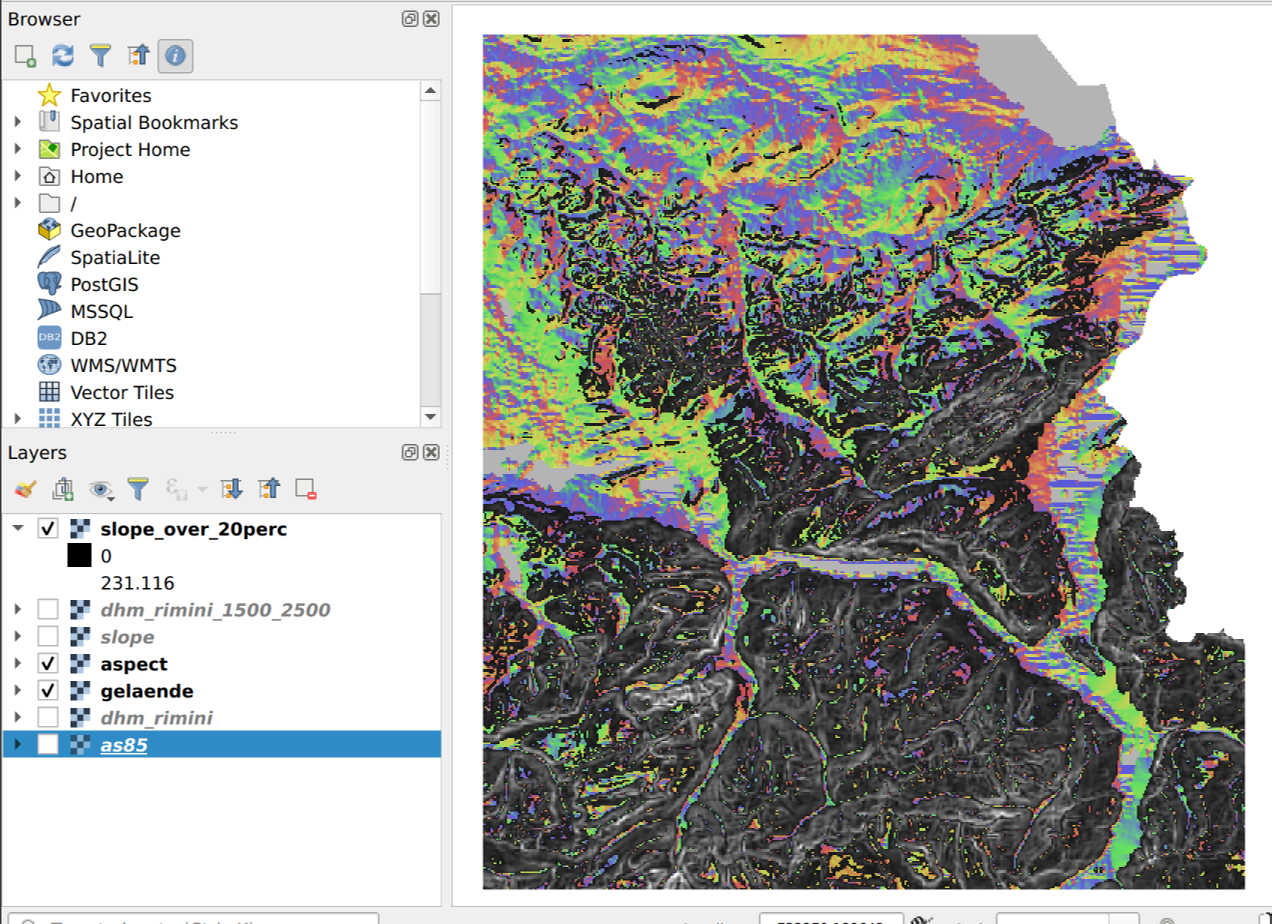
The result is now filtered so that you can see the other layers below:
The same steps - first raster calculator then transparency - you apply now for all further three criteria, as follows:
For the second criterion you start from the layer or
channel “Inclination@01” and save the result in
the exercise data folder under the name
slope_over20perc.tif (Ok is not yet activated).
In this case, use the raster calculator to select all
raster cells that are steeper than 20%.
Then Ok.
For the third criterion you use the layer "Perspective"
(aspect.tif) and filters out all raster cells that lie
between 135 and 225 degrees(i.e. 180 degrees plus/minus 45 degrees).
This will give you all slopes facing south (north is 0° as a reminder).
Save the result in the exercise data folder under the name aspect_135_225.tif.
Then Ok.
For the fourth and last criterion we take the layer “as85”.
The different types of terrain are stored in this as a code (integer).
We are only interested in those areas which have the following uses:
Meadow and farmland, home pastures, spring pastures (Ger. "Maiensässe"),
hay alps, mountain meadows, alpine and Jura pastures.
These correspond to codes 8, 9, 10 and 11.
Filter the layer “as85” according to these codes.
Save the result in the exercise data folder
under the file name as85_sorted.tif.
Remember to set the custom transparency for each layer to 100 percent for the values from 0 to 0 (see Layer Properties).
Try this for all steps. In case you’re stuck, the next chapter describes each step with a solution and screenshots.
Now you’ve made all the necessary calculations.
Now you have to overlay/intersect the four layers.
You use the raster calculator again and combine the four layers
“dhm_rimini_1500_2500”, “slope_over20perc”,
“aspect_135_225” and “as85_sorted” with the logical AND operator.
Name the result good_for_gaemsi.tif and
save it again in the exercise data folder.
Again, you should set the custom transparency
to 100 percent for the values from 0 to 0.
If you want, you can also color this result with a singleband pseudocolor or palette:
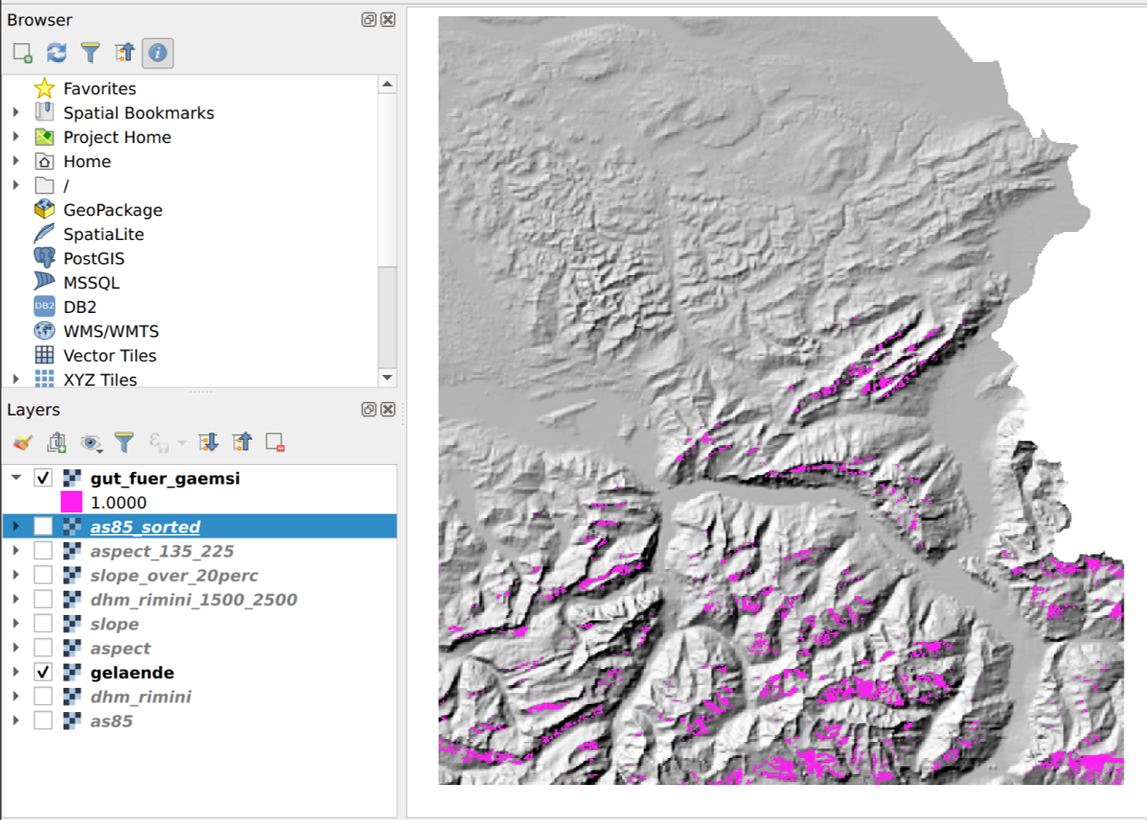
Now we know where the chamois presumably live! At least according to our data and assumptions.
For this exercise are now so far satisfied. But there are still some possibilities for improvement, on the one hand for better readability (e.g. with important places, roads and mountain peaks) and on the other hand with improved analyses where for example the raster cells could be converted into vectors to link the resulting polygons with further data.
Detailed instructions
This chapter is a supplement to the previous chapter, where only the first criterion was explained in detail.
To calculate the other three criteria, we proceed in the same way as for the first criterion. I.e. we first use the raster calculator and then set the transparency of the unneeded values to "transparent".
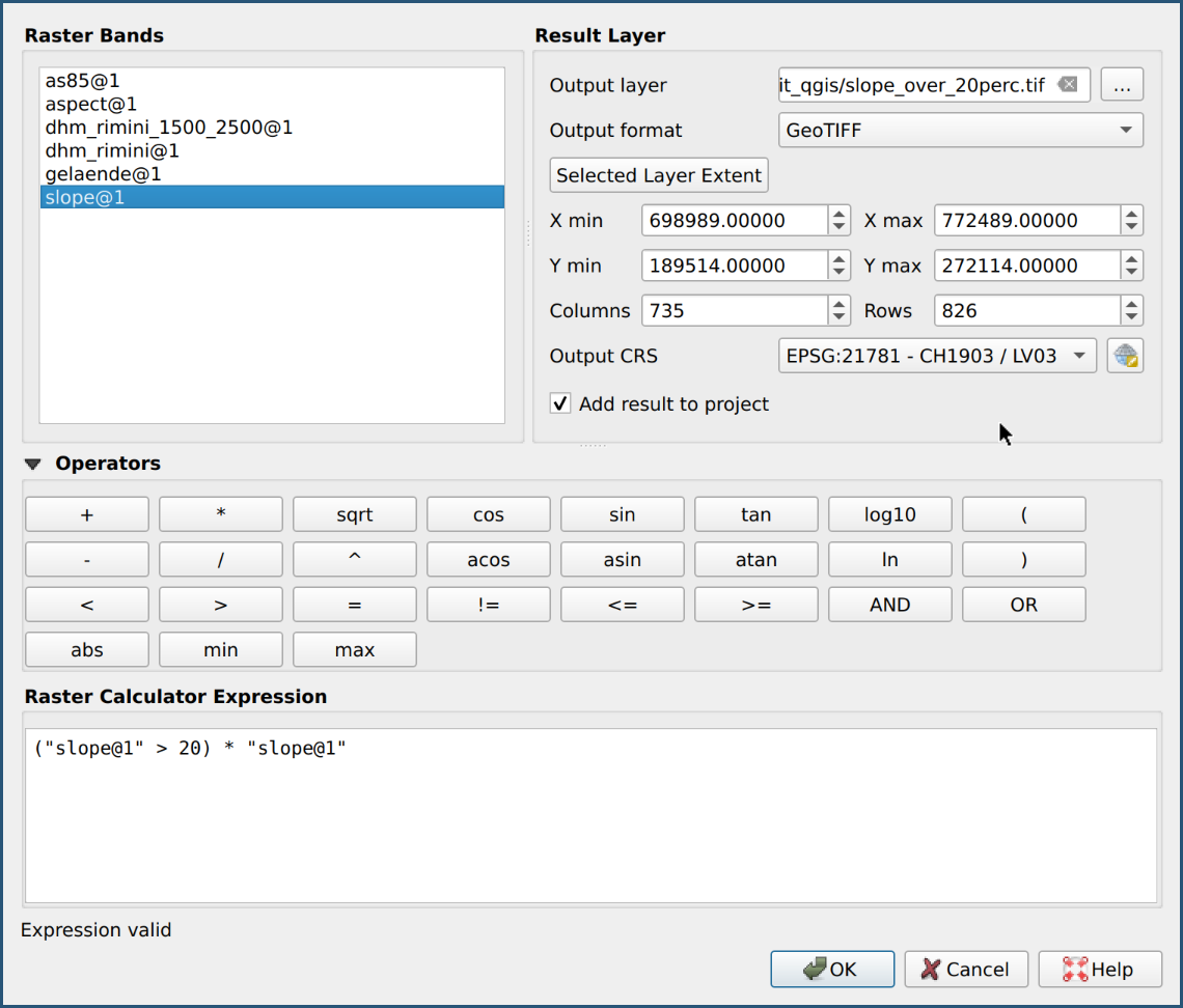
Second criterion (areas steeper than 20%):
Open the raster calculator, select the raster channel “Neigung@1” and enter the following raster expression:
("Neigung@1" > 20) * "Neigung@1"
Then set the transparency of the layer.
The result of the second criterion should be approximately as follows:
Third criterion (southern slope):
In the raster calculator set the output layer aspect_135_225.tif,
select the raster channel "Perspektive@1" and
enter the following raster calculator expression:
("Perspektive@1" >= 135 AND "Perspektive@1" <= 225) * "Perspektive@1"
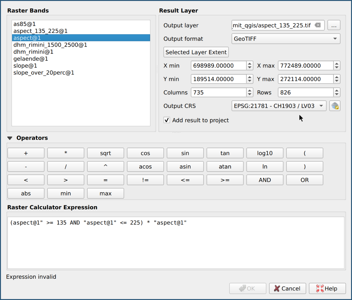
Then set the layer transparency. The result of the third criterion (singleband pseudocolors copied from "perspective") should look something like this:

Fourth criterion (types of terrain):
In the raster calculator select the raster channel
“as85@1”, the output layer as85_sorted.tif
and enter the following raster expression:
("as85@1" >= 8 AND "as85@1" <= 11) * "as85@1"
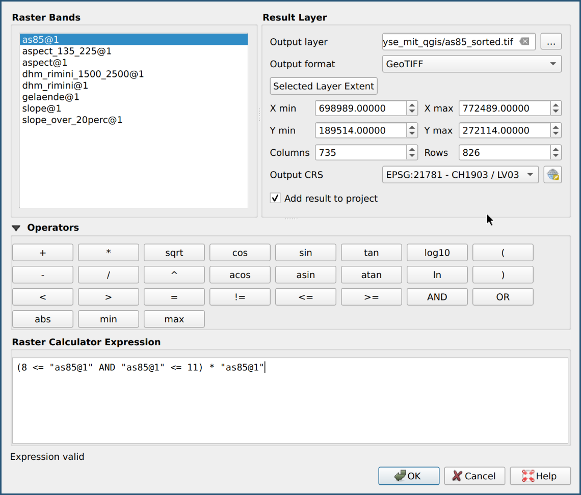
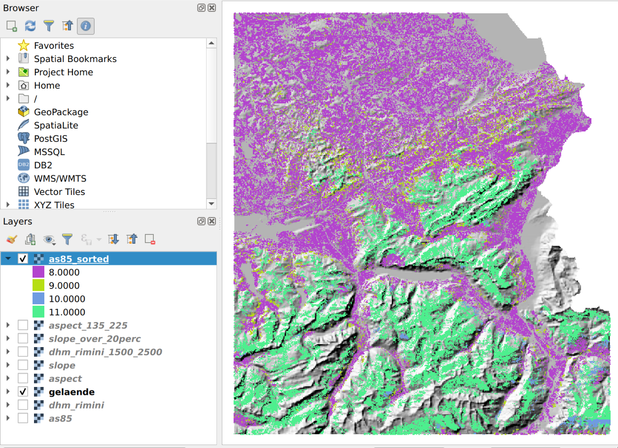
Below is the result of the fourth criterion (palette colors and also with transparency):
Spatial overlay:
Last but not least we calculate the chamois locations with a spatial overlay
(intersection) and save it under good_for_chamois.tif.
Here is the solution for the raster calculator expression:
"dhm_rimini_1500_2500@1" AND "slope_over20perc@1" AND "aspect_135_225@1" AND "as85_sorted@1"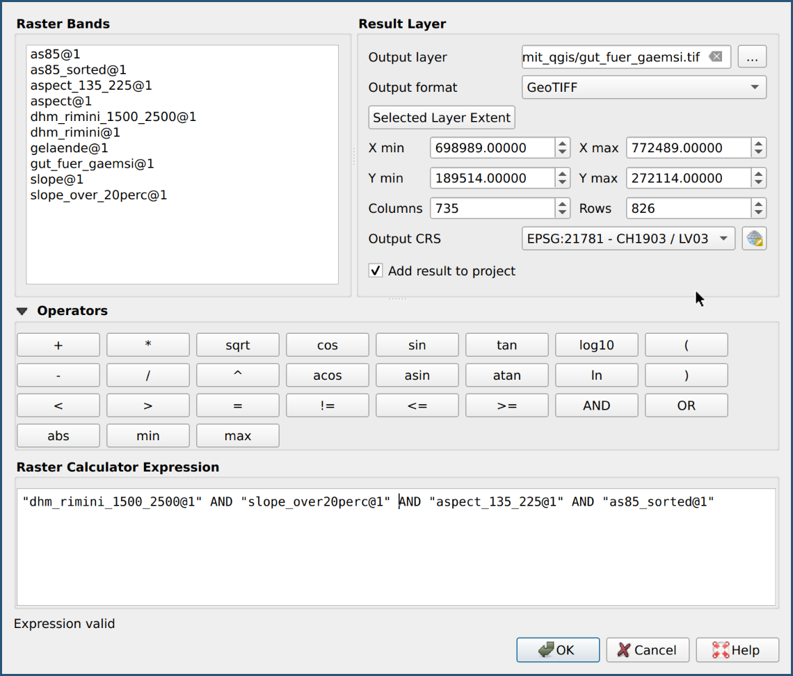
The result is shown at the end of the previous chapter.
■