Joining Tables

OpenSchoolMaps.ch — Free learning materials for free geodata and maps

A worksheet about data handling for interested individuals and teachers

1. Overview

Goals and Objectives

The goal of this worksheet is to explain the following:

Understand what joining of tables is.
Understand the relationships among tables like one-to-one, one-to-many and many-to-many.
Know simple numeric classification algorithms and know how and when to use them by using the desktop program QGIS.

Prerequisites

In order to complete this worksheet, you need the following prerequisites:

Software: QGIS (tested with QGIS 3.4, 64-bit).
Internet access to download data and to eventually install QGIS (download).

On the OpenSchoolMaps website there is a link to download the ZIP file 'Data' ('Daten') which you can find under Weitere Arbeitsblätter zu QGIS 3 und Geoinformationssystemen (GIS) Joining Tables Daten. So please download this file before you start. It contains the following files:

World_Countries.gpkg
CO2_Readings.xlsx
Worldbank_Countries.xlsx
RenewableEnergy_Percentages.csv and RenewableEnergy_Percentages.dbf

If you don’t know QGIS yet, feel free to checkout the our other worksheets on OpenSchoolMaps > "Introduction to QGIS 3 and Geoinformation Systems (GIS)".

2. Introduction

Structured data is modeled in a composite data structure. Structured data is often organized in tables, i.e. in a tabular form. In a tabular data model, there are columns (also known as: field, attributes, cells) and rows (also known as: records, lines, entries). These columns have also a so-called data type, which further describes the content in the column.

An address list is one common example of, structured data in a tabular form, a table consisting of columns e.g. zip which is of type integer (at least in some countries).

In contrast to that there is unstructured data e.g. a free text document which isn’t organized like a table (just a long character string).

Two tables can be linked if both contain at least one column that contains similar data to the other one. These colums, are also referred to as keys, that can establish relationships between various tables. Well-known examples of keys are postal codes or number plates, as these already serve as unique identifiers in their real form. The tables can still be modified and displayed separately from each other. Think of it as a contract that is made between two tables. A column in each of the two tables indicates exactly which row it points to. When data is retrieved from one table, the connected table delivers its data according to this contract.

Keys are identifiers that point to specific entries in a table. That is why they are used to link tables. The most commonly used is probably an id, which gives each entry a unique number.

Then there is the special case where the link goes through a specially enabled attribute. In this case, we talk about Geodata. Geodata is data that has at least one spatial attribute. Such a spatial attribute typically contains a point, a line or a polygon, but it can also be a zip code, a geographic name, geohash code or any other geographic code.

Classification

Classification serves as a vital aid in understanding freshly obtained data. Information alone is not enough to interpret data. This is why we classify data.

Data Types

A data type determines the allowed value range of an attribute. Examples of data types are text or integer. And a typical value range of a four-digit integer - such as a Swiss postal code, which reaches from 1000 to 9999.

The following data types are typically suitable for linking, but of course there are more options:

Number (Integers). Numbers are very often used to link tables. For example, they can be used as ID.
String. Texts can also be used to link tables. For example, you can take a name as a key value.
Date (e.g. date ISO-8601 like 2022-04-01). Data also offers itself as a key for linking. This way, you can break down data according to a date.

Joining Tables

When joining tables, you want to connect data from one table with matching data from another table. To do this, you define a connection point between the two tables, which consists of one column from each of the two tables. This same column does not have to have the same name, but it must have the same data type. By connecting can give new insights on the original data.

In the following example, the two tables can be joined because they share Country as a common attribute. We can use this Column as a primary Key. In this case, the datatype of the key that is used to link the two tables is a string.

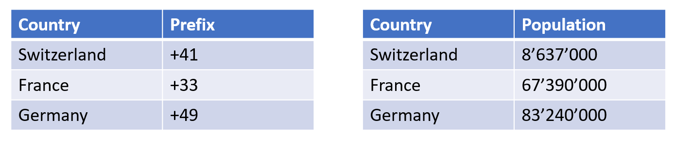
Figure 1. Thes two tables can be joined via Country as this is a common attribute between the two tables.

Relationships

Between two tables, data can be in one of the following distinctive relationships with themselves:

one-to-one (1:1)
one-to-many (1:n)
many-to-many (n:m)

One-to-one and one-to-many will be put to use in the exercise later.

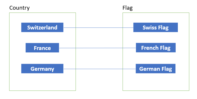
One-to-one (1:1)

One-to-one means that each row in the first table is related to one single corresponding row in the second table. For example, every country has one flag that represents it. In return, each flag is linked to one specific country.

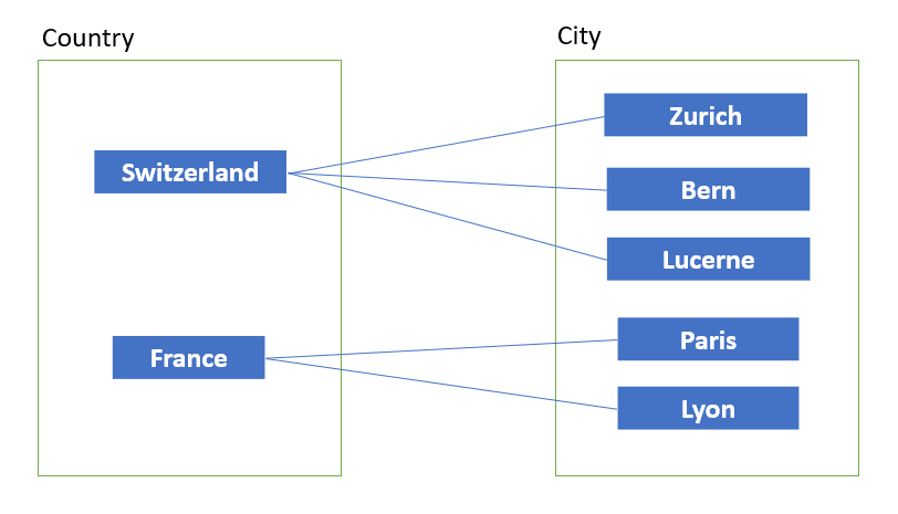
Figure 2. Each country points to exactly one flag and vice versa.

One-to-many (1:n)

One-to-many means that each row in the table is related to more than one row in the second table. For example, every country has multiple cities. In return, each city exists in only one country.

It’s important to know that two equally named cities aren’t considered "the same" city.

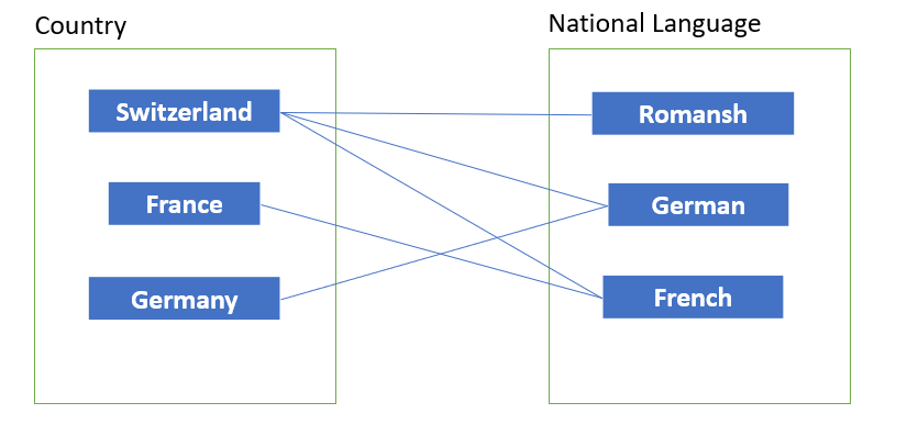
Figure 3. A country can point to multiple cities, but a city can only point to one country.

Many-to-many (n:m)

Many-to-many means that more than one row is related to one or more row in the second table. For example, every country can have multiple national languages (e.g. Switzerland). In return, a language can be the national language of several countries (e.g. French).

Figure 4. A country can point to to more than one national language. A national language can also point to multiple countries.

Terminology

In the following, a few terms are explained again for the sake of understanding:

Table - a table is a collection of related information stored in a format with columns and rows. Tables are basic structures of databases.
Attribute - a component of a table, most of the time it is the field that describes a specific feature of the dataset.
Record - Row of the data table.
Join operation - process of attaching the fields of one table to those of another one based on a common attribute.
Data classification - process of grouping series of data into meaningful categories to enhance the interpretation.

3. Exercises

This part aims at practicing table joining. The goal is to append more attributes to an existing table in the table with spacial data. The newly created layer can be saved, thus creating a new file, or discarded if deemed unsatisfactory.

Exercise 1.1 - Information Gathering via Join

In this exercise, we will go through the process of joining tables to gather as much knowledge from numerical sets as possible.

This is the data needed for this exercise:

World_Countries.gpkg
CO2_Readings_World.xlsx
Worldbank_Countries.xlsx

Here, the numerical data consist of CO2 emission values per country saved in an MS Excel sheet. The context is provided by another file that contains the list of every country’s population. The project we’re working with has a list of world countries. Each of these files alone holds a small piece of information. After merging these datasets, they provide enriched and interpretable data. In this case, that would be the amount of CO2 emissions and the population of all countries in a spatially enabled format.

A country’s population can be an explanation for its high / low CO2 emissions. When we’re done creating this new larger table, we will move on to the second part of this exercise: data classification. There, we’ll group data into relevant categories in order to enhance the interpretation even further.

Downloaded data might already include a spatial component like human population in various cities, but to use the data in QGIS, they need to be attached to the already existing dataset. This is where joining tables comes in handy because both data files can be connected to reveal more information.

Open QGIS and in the project select Project New to create a new QGIS project.
Add the World_Countries.gpkg file to the project by dragging it from its file location onto the layer section on the left side of the QGIS editor.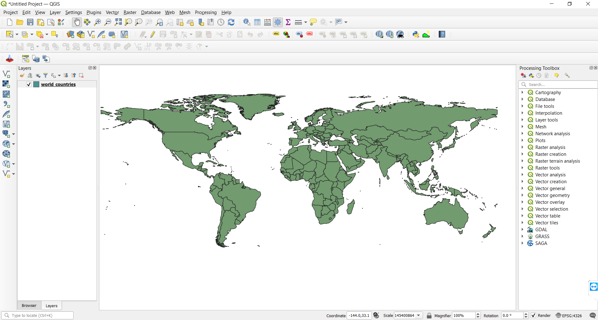

Figure 5. This is how everything should look after World_Countries.gpkg has been imported.
To examine the attribute table of the layer you just imported, right-click on it and choose: open attribute table

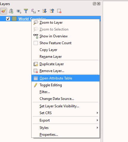Figure 6. Context menu for opening the attribute

You should now be able to see the data from World_Countries.gpkg. There should be three columns: REGION, NAME_12 & C_NAME.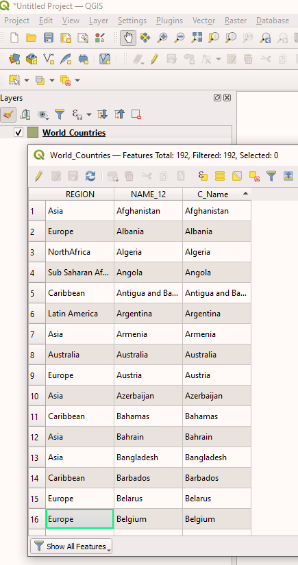

Figure 7. Attribute table displaying the data from World_Countries.gpkg
Close the attribute table.
Now we’re ready to add additional data to the countries. Click on: Layer Data Source Manager

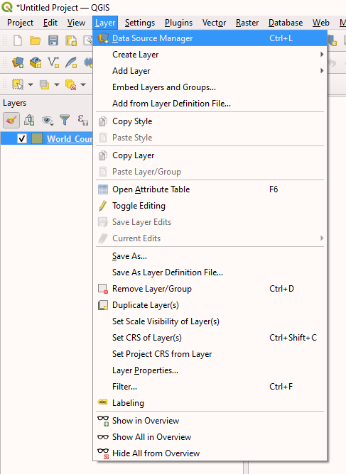Figure 8. Context menu for opening the Data Source Manager.

In the Data source manager, select Browser in the sidebar to see your folder tree. Look for the folder where you saved CO2_Readings_World.xlsx: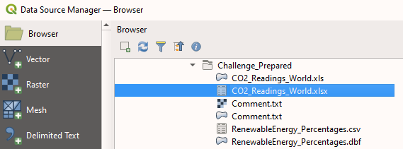

Figure 9. QGIS’s Data Source Manager

Double-click on the file to add it to the layers in your project. Afterwards, you can close the Data Source Manager.

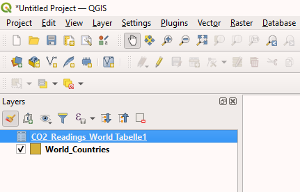Figure 10. CO2_Readings_World.xlsx was used to create a new layer.
Right-click the newly added layer and open its attributes. Feel free to explore the data to familiarize yourself with it.
Close the attribute table.
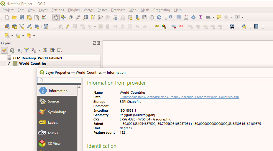Right-click on the World_Countries layer Properties Layer Properties window:

Figure 11. Layer Properties window.
To configure the joins for the table, choose Joins from the sidebar.

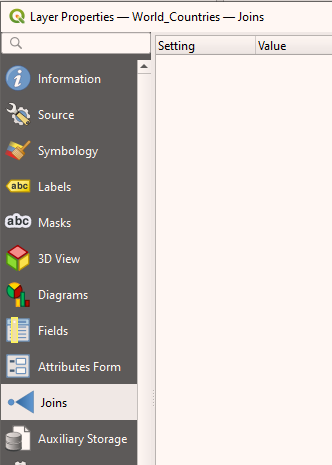Figure 12. Joins in Layer Properties sidebar
Click on the green + icon in the bottom left corner of the Join window. This will open the Add Vector Join window.
Select C_Name attribute in Join Field and Target field menu. Check Custom field name prefix and add a type "joined" into the text box.

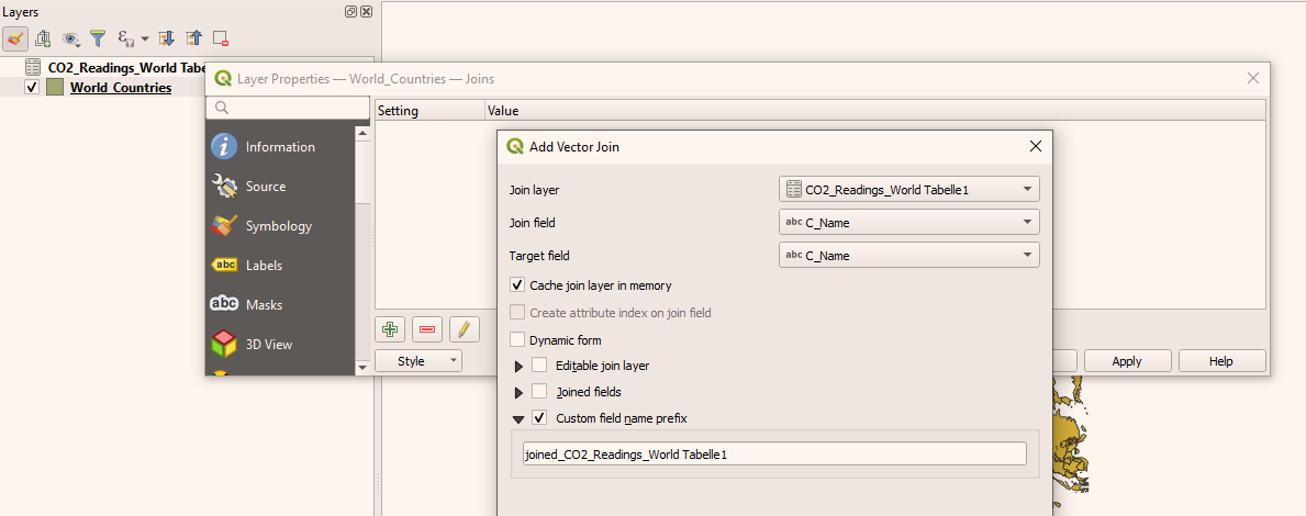Figure 13. All attributes were selected and the new name was given.

Click OK.
Expand the list by clicking on the black triangle next to Join layer to see the summary of the operation.

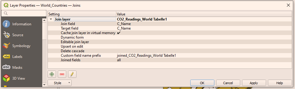Figure 14. The summary of the joining table operation.

Click OK.
Reopen the attribute table of the World_Countries layer.

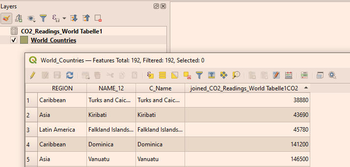Figure 15. New joined attribute table of the World_Countries layer
Repeat steps 5 - 13 and add another spreadsheet file: Worldbank_Countries.xlsx to the project and join the tables reusing the field name as a connection.
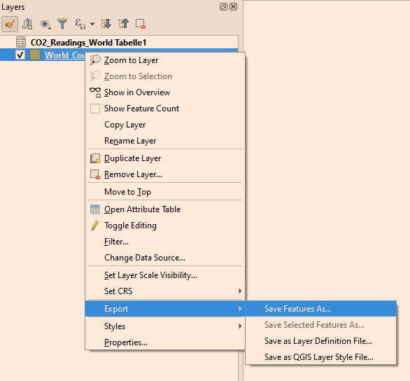The new tables are temporarily saved within the project. To save them to disk you have to click on World_Countries layer Export Save Features as …

Figure 16. How to save the new joined tables layer

Select GeoPackage as format.

Set the filename to world_countries_co2.

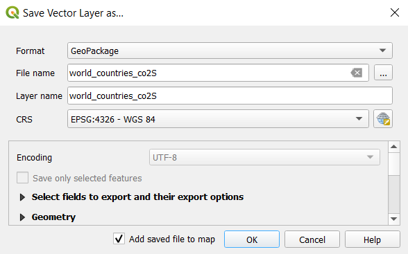Figure 17. Settings for saving the new GeoPackage.

Double-check if Add saved file to map is ticked. If it is ticked, you can proceed by clicking OK. The message on the green field: “Layer Exported: Successfully” should be visible above the map in the main window.
Remove the original layers World_Countries, CO2_Readings_World and Worldbank_Countries. Click on each layer and choose: Remove layer.
You can now save the project in your folder.

Exercise 1.2 - Further Practice Joining

Now you should be ready to try to join tables for yourself:

Join the tables from the original table in the World_Countries.gpkg file, but use CO2_Readings_World.xlsx this time. Try not to use the tutorial as a guide.

4. Exercises (Bonus Part)

While it may be easy to obtain data, it’s rather hard to interpret their meaning. Therefore, in this chapter, we will classify and visualize our now processed data. So let us take a look at how to do exactly that; how to reveal additional information from table datasets.

Exercise 2.1 - Classify Data with Color

In this exercise, we will make joined data visible by using color to visualize the data.

This is the data needed for this exercise:

World_Countries.gpkg
CO2_Readings_World.xlsx
Worldbank_Countries.xlsx
1. Open the project from Exercise 1.2 in QGIS:
Now you can decide whether you want to use:
Project Open
Project Open From or
Project Open Recent (This is the most convenient option if you’ve been working on your project recently).
1. Open the layer styling panel and choose Joined Tables layer as the target.
  
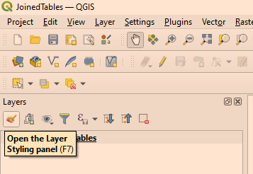  Figure 18. Where to find Layer Styling Panel
2. Move to Layer Styling Panel and set:
Graduated renderer
Symbol value to joined_CO2
Leave the legend format default
Change color ramp to any color you like
Mode to Equal Count (Quantile)

Once you’re done, click on classify in the bottom left corner of the window. Depending on your choice of color, the result should look something like the following picture:

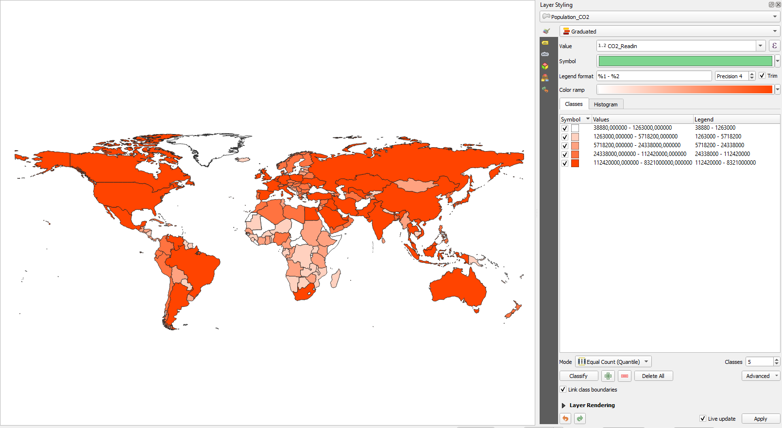Figure 19. Result of applying the Equal Count classifier to the C02 value in the joined table

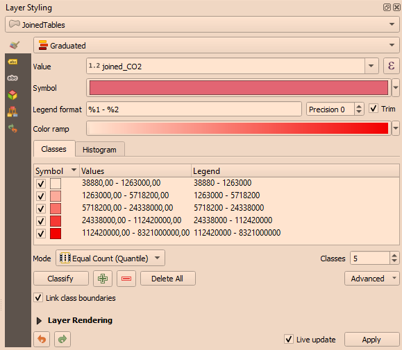Figure 20. Classification settings in detail
1. Repeat step 3 for the world population value. Do not forget to change to a different color, or else you won’t be able to tell it apart from the CO2 layer.
Figure 21. Result of applying the Equal Count classifier to the world population value in the joined table

Some information about the data modes or classificators for advanced users:

Equal count (Quantile):

Sample quantiles are produced corresponding to the given probabilities. The smallest observation is represented by 0 and the highest by 1.

Equal Interval:

Divides the range of attribute values into equally sized classes. The number of classes is determined by the user. The equal interval classification method is the best for continuous datasets such as precipitation, temperature or population.

Logarithmic Scale:

Way of displaying numerical data over a very wide range of values in a compact way - typically the largest numbers in the data are hundreds or even thousands times larger than the smallest numbers.

Natural Breaks (Jenks):

Jenks is a type of "optimal" classification scheme, finding class breaks that (for a given number of classes) will minimize within-class variance and maximize between-class difference.

Pretty Breaks:

Rounds each break-up point up or down. So instead of having a breakpoint at 599.85, it will have it at 600.00

Standard Deviation:

Finds the mean value, then places the class breaks above and below the mean at intervals of either .25, .5 or 1 standard deviation until all data values are contained within classes. Values that are beyond three standard deviations from the mean are aggregated into two classes: greater than and less than the mentioned standard deviations.

You can change the number of classes as well. Find the number that best represents your understanding of the data.

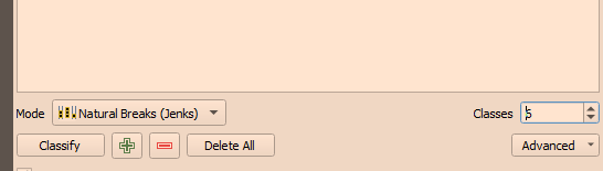Figure 22. Number of classes can be found in the bottom right corner
To highlight the differences among the data in various classes, it is sometimes useful to use different colors. The option that allows us to do this is called RdBu color ramp:

Click on:

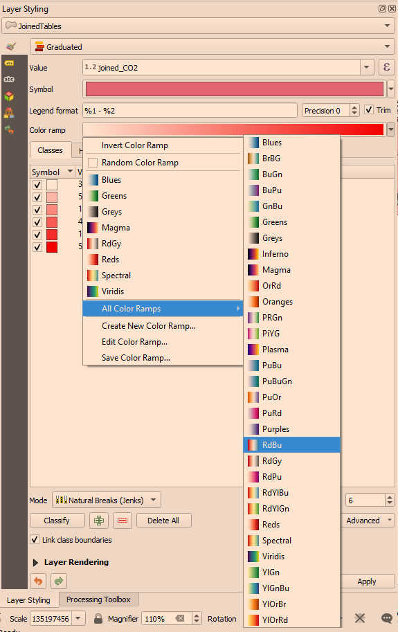Color ramp color All Color Ramps RdBu

Figure 23. RdBu option

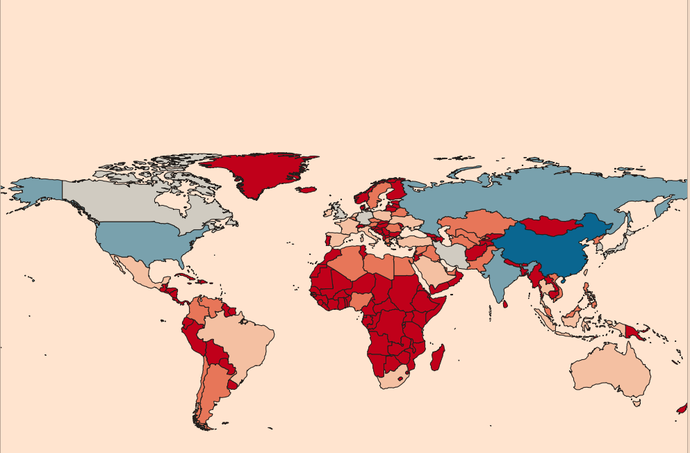Figure 24. RdBu for 6 classes and Natural Breaks (Jenks) classification mode

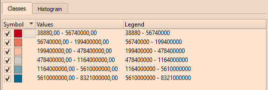Figure 25. Default legend

Type into legend to replace the strings with words:

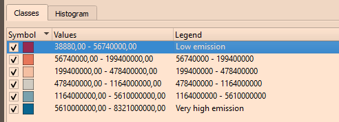Figure 26. Modified legend

Exercise 2.2 - Join Additional Data

In the data folder, you will find a file: RenewableEnergy_Percentage.csv

Use this file as additional data to be joined to your table (you should repeat the steps from part 1 of this tutorial). Do the classification. Describe the results and explain the usage of the number of classes and classification modes you have chosen. Joining additional data sometimes is also being called Data Enrichment.

5. Conclusion and Outlook

To sum up, this tutorial aimed at explaining how to join tabular data. The goal of doing the exercises in QGIS was to learn about the methods that allow the user to join tables of data and thus create new ones with extended context. The basic introduction about the various relationships among the data, like one-to-one, one-to-many and many-to many, can be studied further to deepen the knowledge about datasets. The part devoted to data analysis taught the essentials of data classification. The additional information about the classification algorithms gives a comfortable head start that can be further increased by the student individually. This tutorial serves as a guide on importing data into a QGIS environment, joining them into a new table, classifying them and lastly analyzing them.

The many-to-many relationship was not dealt within the exercises here. However, it is possible to use many-to-many relationships in QGIS. If you want to learn more about that, you can do so in the QGIS Doc.

Additionally, if you want to learn more about joins in databases and how to use them, you can find more under the keyword SQL JOIN.

Open questions? Feel free to contact OpenStreetMap Schweiz or Stefan Keller!

Freely usable under CC0 1.0