Spatial analysis with hectare grid data: visualization of statistical information of a Swiss municipality with hectare grid data
OpenSchoolMaps - Free learning materials on free spatial data and maps
Worksheet for self-studying, students, schoolchildren and teachers on upper secondary level (secondary schools and grammar schools).
Goals and general information
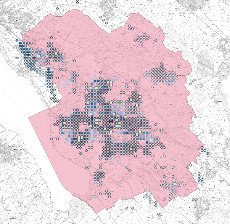
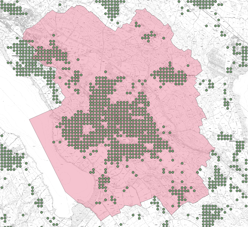
The aim of this exercise is to show the spatial distribution of the resident population using the example of the municipality of Uster in the canton of Zurich. In addition, the spatial distribution of the schools should be shown and terms such as hectare grid, spatial density and classification should be explained.
Figure 1 below shows one possible result of this worksheet.
After completing this worksheet, you will be able to
-
Understand the data sources and data structure of hectare grids;
-
Read data in “Delimited Text” format CSV with QGIS and save it as a layer (in the Geo-Standard format GeoPackage);
-
Classify the hectare grid data with QGIS functions;
-
Symbolize and visualize the hectare grid data.
General information:
-
Time required: This exercise takes approx. 1 hour, depending on your previous knowledge.
-
Keywords: spatial data analysis, classification, GIS, QGIS, CSV, GeoPackage.
Introduction
The concept of hectare grid, spatial density and classification
It is important to know where people live and how many there are. This has been the case since the Old Testament. Every country carries out censuses, including the Swiss Federal Statistical Office (BfS), which keeps statistics on the population and households. For the publication, the BfS chose a data structure with points that are managed in a regular grid with a width of 100 m. The measurement unit is called “hectares” and each grid cell is 100 x 100 meters. This results in a so-called "hectare grid".
NOTE: The hectare (singular), is a unit of measurement of the area with the unit sign ha. The hectare is mainly used in agriculture and forestry and corresponds to an area of 10,000 m², for example, a square field with side lengths of 100 meters.
In addition to the statistics of the population (called the hectare grid BfS STATPOP), the BfS publishes further interesting geodata of buildings (GWS), companies and employees (STATENT) as well as of land use and land cover (area statistics, NOAS).
The hectare grid data structure was also adopted by other data providers, such as the Office for Statistics of the Canton of Zurich and the Institute for Software in Rapperswil, including schools and shops and potentially over 1000 so-called points of interest (POI). The latter data set is called “hectare grid OSM”.
Questions of spatial analysis with hectare grid data.
Typical spatial analysis questions that can be answered with such statistics:
-
"What is the spatial distribution of the population, i.e., the population density (source: STATENT)? In other words: Where do more and where fewer people live within a municipality?".
-
Thanks to the GIS layer principle (see GIS basics), this layer can be overlaid with other layers. An additional question could therefore be: "What is the spatial distribution of schools there?" (source: hectare grid OSM).
-
Given by these two levels - and it can now be asked: "Do the two distributions correlate with each other?". i.e. "Are there many schools where there is a high population density? Are there areas where schools are lacking?"
A spatial density is typically visualized with brightness, so the darker an area is, the higher the population density is, for instance. To increase comparability of analysis and visualization, we need to classify the data - in this case, persons per hectare (such as 0-50 persons per unit area as Class 1, then 51-100 as Class 2, then 101-150, etc.) This classification results in a more readable map.
Tools and procedure
As an aid for this worksheet you need an installed QGIS (tested with QGIS 3.14.15) as well as the data basis, which will be presented shortly.
The further procedure is as follows:
-
The data bases at a glance.
-
The hectare grid BfS; Reading in the text / CSV file.
-
The hectare grid OSM; Reading in the GeoPackage file.
-
Classification of the hectare grid data through symbolization.
Data basis
Before the actual input data are presented, here is the basic map and the basic data set, which are used for orientation and limitation:
-
A basic map for orientation as a raster-tile service.
-
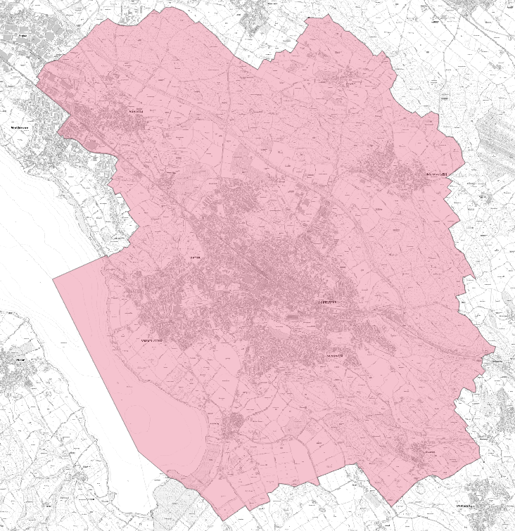
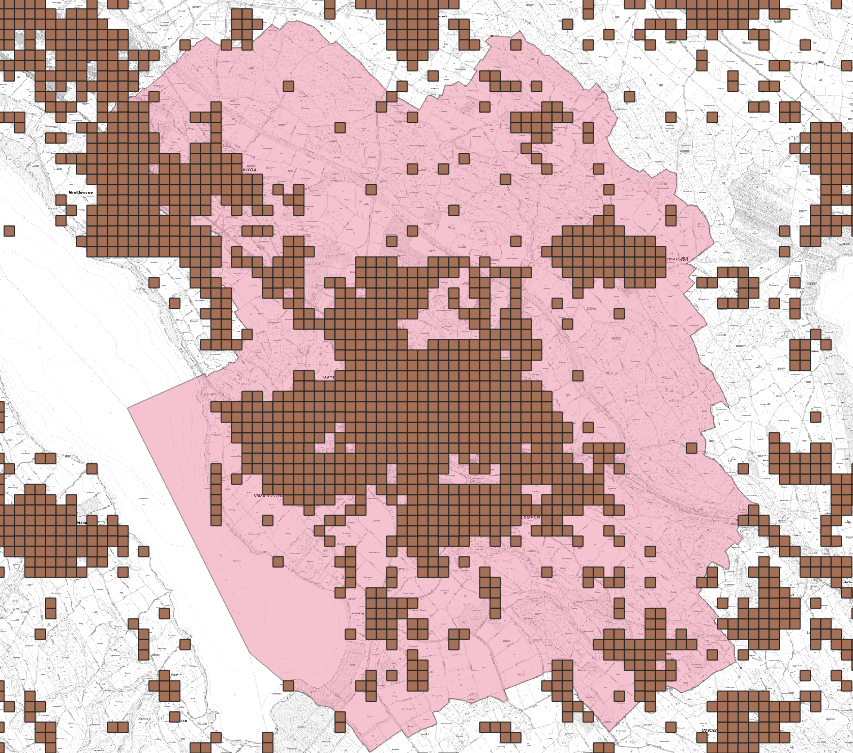
File “Gemeindegrenzen_Uster.geojson” in GeoPackage format (polygon) the municipal boundaries of Uster; see figure 2.
These are the actual input data:
-
“STATPOP2019” file, in CSV (Point) format, the FSO’s population statistics from 2019.
-
File “hectare grid_CH-ZH.” in GeoPackage format (polygon) of the schools from OpenStreetMap.
BfS hectare grid
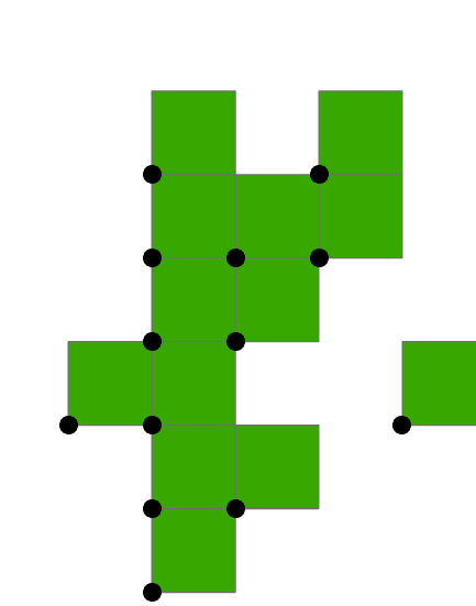
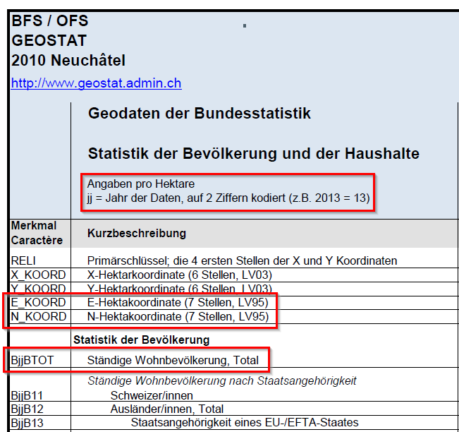
A section of the point data set "Statistics of the population and households 2019" (STATPOP) from the Federal Statistical Office (BfS) is available as working data (STATPOP2019.csv). The data on the population and households is aggregated on a grid with a grid width of 100 m. This means that the attributes are only available per hectare grid cell. Since STATPOP is a point data set, it is important to know which hectare area this information relates to. From the metadata, it can be seen that each point is a southwest corner point of a hectare grid cell, respectively. (see "be-d-00.03-10-STATPOP-v110.pdf").
In addition, the metadata also show that the attributes "E_KOORD" and "N_KOORD" are the E and N coordinates of the new reference frame LV95. In addition, the attribute "B19BTOT" is also significant for this exercise. This corresponds to the total population of permanent resident within the hectare grid cell (cf. 'be-b-00.03-10-STATPOP-v120.pdf').
hectare grid OSM
An excerpt from "hectare grid OSM" is available as a further data set for the exercise (hectare grid_CH-ZH.gpkg). It is an excerpt from OpenStreetMap aggregated on the hectare grid. The hectare grid is compatible with that of the BfS data.
There is also a variant with polygons instead of points. The polygons correspond to one hectare grid cell. The advantage of this is that it makes spatial analysis and visualization even easier because the polygon effectively represents a cell. This is in contrast to points, which are “representative” for the cell.
For the present exercise the attribute "schools" is used, which shows how many schools there are in a certain hectare grid cell.
Exercises
Preparation: Create the project file and load the input data
You can find all the data required for the tasks in the source directory on OpenSchoolMaps.ch.
-
Navigate to the directory with the data.
-
Open QGIS.
-
Make sure that the project settings of QGIS also have the coordinate reference system LV95 (EPSG: 2056). (see bottom right corner in QGIS)
-
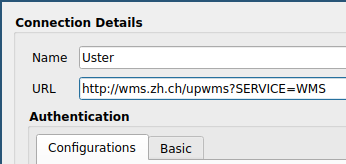
Load base map. i.e. general plan of Canton ZH URL: http://wms.zh.ch/upwms?SERVICE=WMS. ( > new > "see Fig. 7" > connect > adapt coordinate system if necessary > add)
Move layer down in the project.
-
Load the file
Gemeindestrenzen_Uster.geojson. Optional: If you want the municipal boundaries for another location, you can get the data with these three steps.Step 1: Go to www.osm.org and search for the location you want. Look for the relation id of the place, e.g. with Uster this is directly under the name in brackets (1682225).
Step 2: Go to http://overpass-turbo.eu/?template=type-id&type=relation&id=1682225&R and enter the id of the location you are looking for at the place "relation (…)" in brackets.
Step 3: After the Execute click on the Export. Select "Save as GeoJSON" by clicking on the underlined word Save.
-
Save the QGIS project under the name
hectare grid data_Uster(.qgz).
Task 1: Load and extract the hectare grid OSM
In this task the polygons of the hectare grid are extracted and filtered.
-
Load the file
hectare grid_CH-ZH.gpkg(GeoPackage). (This was downloaded from https://drive.switch.ch/index.php/s/CrHsRJeq5yZbEin. In this downloaded file, you will also find the hectare grid for the other cantons in Switzerland.). Note that this data is only available in the original point data structure (and not as polygons such as hectare grid OSM). -
Extract all hectare grid cells in the layer
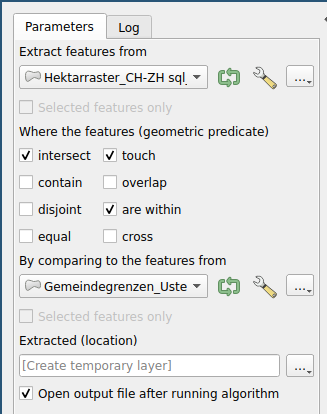
hectare grid_CH-ZH.gpkg, which come to lie within the municipality area of Uster or which intersect with the municipality area. To do this, open the Processing Toolbox. ( ) (See Fig. 8) -
Save the extraction as a layer under the name "Hectaregrid_Uster".
-
In the newly created layer "Hectaregrid_Uster", filter all hectare grid cells in which at least a school is available ( filter with the Provider Specific Filter Expression “schools > = 1”; Select ). This filtering is necessary because the hectare grid data originally contain a cell everywhere that contains either at least one school or one shop (or another POI).
-
Save the filtering under the name "Hectaregrid_Uster_schools". This dataset only contains hectare grid cells, which also contain schools.
Note: The data used here cover the whole of Switzerland. A completely different administrative unit can be chosen instead of Uster.
Now you should have a layer "hectare grid_Uster_schools" in QGIS. At this point in QGIS click on or use the shortcut (Crtl + S).
Exercise 2: Representation of the school density in Uster
In this task, the school density in Uster is shown with a classification.
-
Open the Layer design window, change Single symbol to Graduated and classify the layer "Hectare grid_Uster_schools" with the attribute schools. Work out a classification of the data that makes sense for you.
-
Assign a color gradient to the classes (e.g. from light green to dark green).
-
Make the layer with your symbolization a little transparent so that the base map is also visible.
-
Create a map layout with a legend and export it as a PDF (
School_Uster.pdf). ()
Task 3: Loading the BfS hectare grid
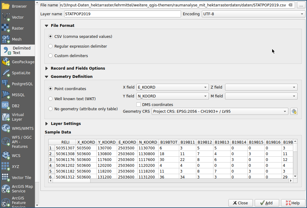
This task shows how to add a .csv file as a layer in QGIS.
The STATPOP2019.csv file can be found in the files folder ( downloaded from https://www.bfs.admin.ch/bfs/de/home/dienstleistungen/geostat/geodaten-bundesstatistik/gebaeude-wohnungen-haushalte-haben/bevoelkerung-haushalte-ab-2010.assetdetail.14716365.html ).
Load the file STATPOP2019.csv with menu .
As described, the E_KOORD and N_KOORD attributes contain the coordinates of the new Swiss coordinate reference system LV95 (EPSG: 2056).
Exercise 4: Representation of the population density of Usters in classes
In this task the population density of Uster is determined by extracting and classifying.
-
Preparation: Provide the municipality of Uster (
Gemeindegrenzen_Uster.geojson) with a buffer 100m (0.003 degrees) and name the layer accordingly: "Municipal_boundaries _Uster_100_Buffer ". (As in exercise 1, open the Processing tools and search for Buffer) -
Extract the hectare grid data within the municipality boundaries: Search as in task 1 Extract by position. Select the layer "STATPOP2019" as Extract objects and the layer "Municipality limits_Uster_100_Buffer" as By comparison with objects. (Select location of objects: cuts, touched and are within, as in Fig. 8) Save your cut as a layer under the name "STATPOP2019_Uster".
-
Classify: Choose Graduated for the "STATPOP2019_Uster" layer and classify it using the "B19BTOT" attribute (stands for "Population 2019 Total"). Work out a classification of the data that makes sense for you in at least 3 and a maximum of 7 classes. Use a gradient (e.g. from light blue to dark blue).
-
Improve symbolization: Make the layer with your classification a little transparent so that the information on the base map can be seen again.
-
(Optional: create a map layout with a legend and export it as a PDF, e.g. as a file
Residential_population_Uster.pdf) (see task 2).
Conclusion
The following data must now be available:
-
Map in PDF format showing the spatial distribution of the resident population in Uster including legend (map layout).
-
Map of the spatial distribution of the schools in Uster in PDF format including legend (map layout).
Summary
In this worksheet you learned how to use hectare grid data to analyze and visualize statistical spatial information for a Swiss municipality.
There are other worksheets on OpenSchoolMaps, especially for spatial analysis. The worksheet Introduction to Table Joins and Classification is planned.
Thanks
Many thanks go to Ms.Oiza Otaru from the Institute for Spatial Development (IRAP) from the OST campus in Rapperswil who has designed this exercise.
Have questions? Contact OpenStreetMap Switzerland (info@osm.ch) or Stefan Keller (stefan.keller@ost.ch)!
![]() Freely usable under CC0 1.0
Freely usable under CC0 1.0