Exercise: Editing and visualizing photos with coordinates
OpenSchoolMaps.ch - Free learning materials for free geodata and maps
A worksheet for self-studying and students
Overview
Photos with metadata
Digital photos often contain hidden additional information, so-called "metadata," in addition to the actual image data. Examples include the time the photo was taken, the name of the camera’s manufacturer, or detailed information about where the snapshot was taken.
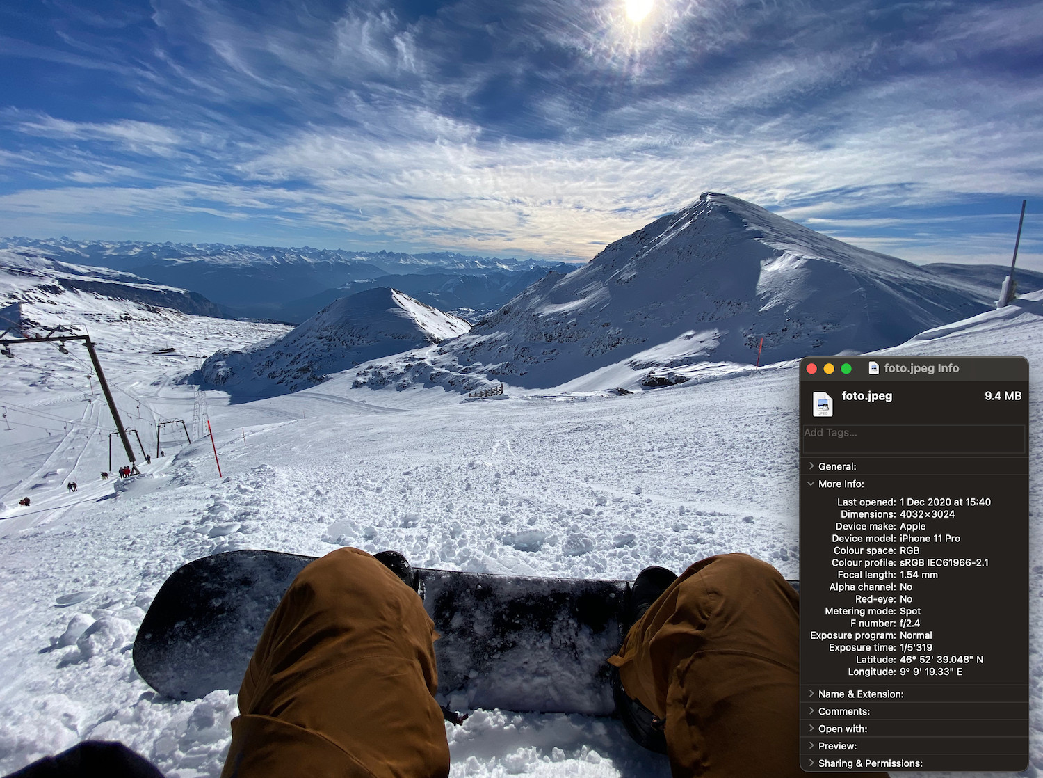
We refer to the information about where a photo was taken as a "geotag". The term "tag" comes from English and means "label". Together with "geo" for "geographic", this results in the "geographic tag". The geotag consists of at least the position (latitude and longitude) of the location where the picture was taken, but can also include other details such as the photographer’s shooting direction.
| If you are interested in more detail about how such metadata is stored for a photo or want to know more about the different types of additional information, the Wikipedia page on "Exchangable Image File Format" (EXIF) is a good place to start. |
In the past, digital photos were often geotagged "by hand": A photographer always had a small GPS receiver with him, which recorded his position and the current time. With a georeferencing program, the photographer could later add a geotag to his photos on his computer: To do this, the program must match the time a photo was taken with the recorded position from the GPS receiver and store the information in the photo’s metadata.
There are also photo cameras that have a built-in GPS receiver or allow an external receiver to be connected via a cable. In both cases, the camera automatically determines the current position and saves it when a photo is taken. Therefore, additional georeferencing work is not necessary.
If you take a photo with a modern smartphone, it is highly possible that your photo will be automatically saved with a geotag - If the function is activated in the privacy settings, the camera automatically uses the built-in GPS receiver and compass to create a geotag.
| If you own a smartphone but still prefer to take photos with a regular camera, you don’t have to give up geotags! With a GPS logger app, you use your smartphone to record your position and then geotag the photos from your camera with a georeferencing program. GPS logger apps are available for iOS and Android smartphones: search for apps with the keywords "gps tracker photo" or "gps logger photo". |
Objectives
With this worksheet you will learn step by step how to import, arrange and display photos with geotags in QGIS. Later on you will find out how to display the photographer’s line of sight on your map.
Before you start.
-
Time required: This exercise will take at least 30 minutes if you already know a bit about QGIS.
-
Prerequisites:
-
A computer with QGIS 3 installed. (This exercise was prepared with QGIS 3.14.15-Pi).
-
You have downloaded and unzipped the map material and photos. Here you find:
-
A folder
photoswith 12 photos, including geotags. -
A GPKG file 'Basel-Innenstadt.gpkg', which contains maps of the Basel city center.
-
-
Tasks
On a trip to Basel you took some photos in the city center. Some months later, you find the snapshots on the memory card of your photo camera, but forgotten the details. While going through the shots with a friend, you start discussing where exactly in Basel the photos were taken.
After some back and forth, you want to know exactly: Since your photos fortunately have geotags, you decide to display all the shots clearly on a map of Basel’s city center.
Preparation
-
Launch QGIS and start with an empty project
-
Set the coordinate reference system for your project to EPSG: 2056. (Tip: Click on the corresponding button at the bottom right of the QGIS window, to open the KBS settings.)
-
Add
Basel-Innenstadt.gpkgas GeoPackage data source to your project. (Tip: Click with the right mouse on GeoPackage in the Browser and select New connection.) -
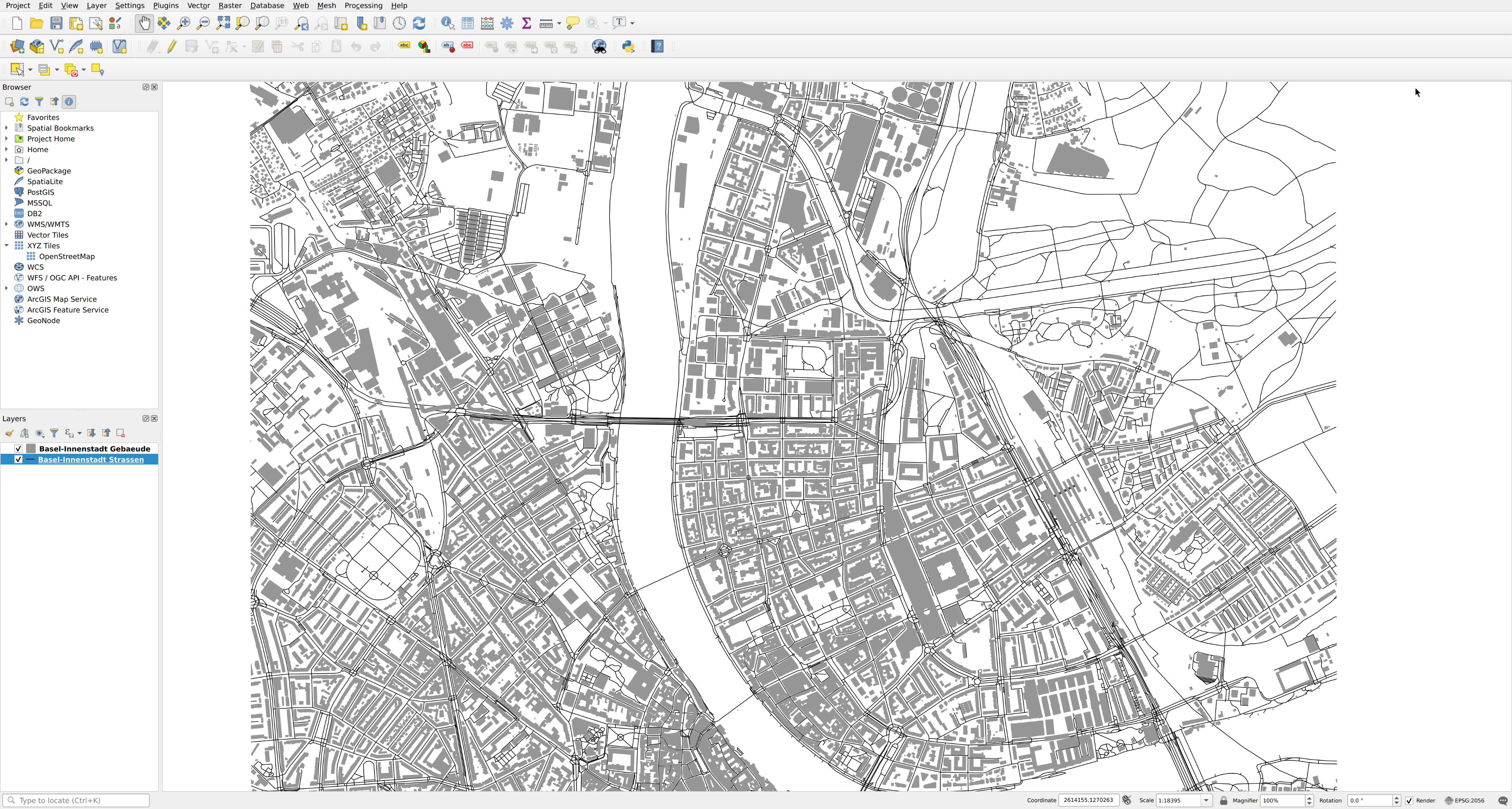
The GeoPackage of Basel city center contains two layers: "Streets" and "Buildings". Add both layers to your project. (Tip: Click with the right mouse button on a layer and select Add layer to project.)
-
Set the display options for the street and building layer according to your taste. We chose black for streets and gray for buildings. (Tip: In Chapter 3 "Introduction to QGIS 3: Acquisition and Management of Data" you will find further information on how you can influence the display of layers in QGIS.)
After completing the preparation, you are now ready to import the photos into QGIS for the first task.
Task 1: Import photos
QGIS provides you with a special tool to import photos. The tool Import geotagged photos can be found in the Processing tools. To show these, click on the button symbol in the Toolbox.
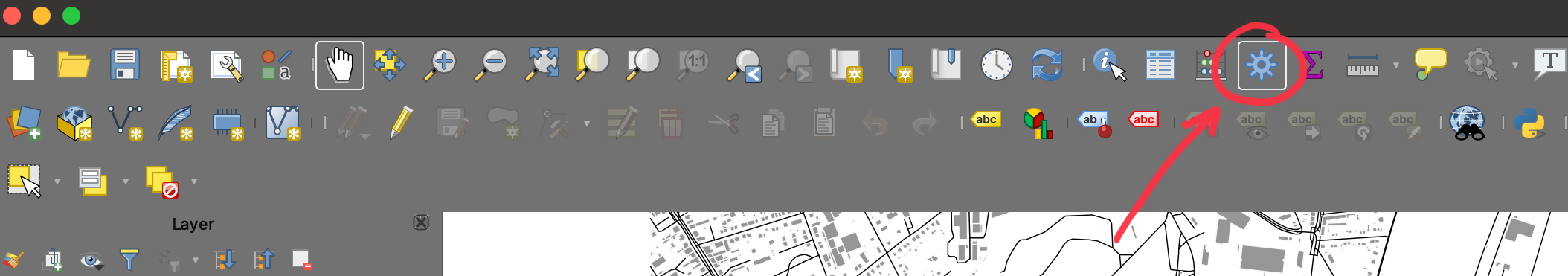
A new area with a list will appear on the right edge of your QGIS window. To open the tool import geotagged photos, click in the processing tools on the arrow to the left of the term vector generation. Do you now see the entry import geotagged photos? Double-click on it:
|
Alternatively, you can enter the term "Geogetagged" in the "Search" field
|
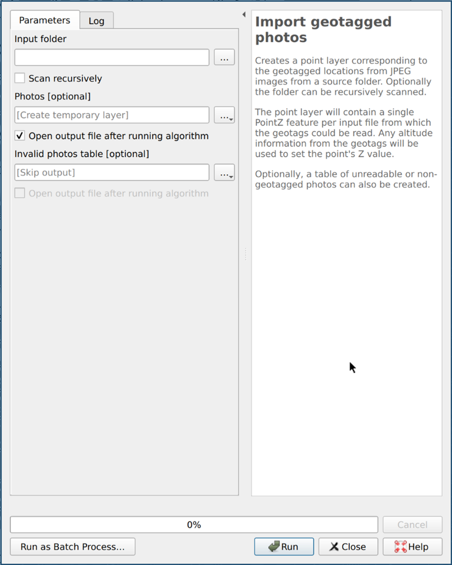
Click on the button Browse ![]() and select the folder
and select the folder photos from the exercise files.
Next to the Photos [optional] field, click the Browse ![]() again
and select Save to file.
Choose any file in which the locations of the photos should be saved.
again
and select Save to file.
Choose any file in which the locations of the photos should be saved.
You can ignore the rest of the settings in the dialog for the moment. When you’re ready, click the Run button in the lower right to import all the photos. After the import is complete, click on Close to close the tools dialog.
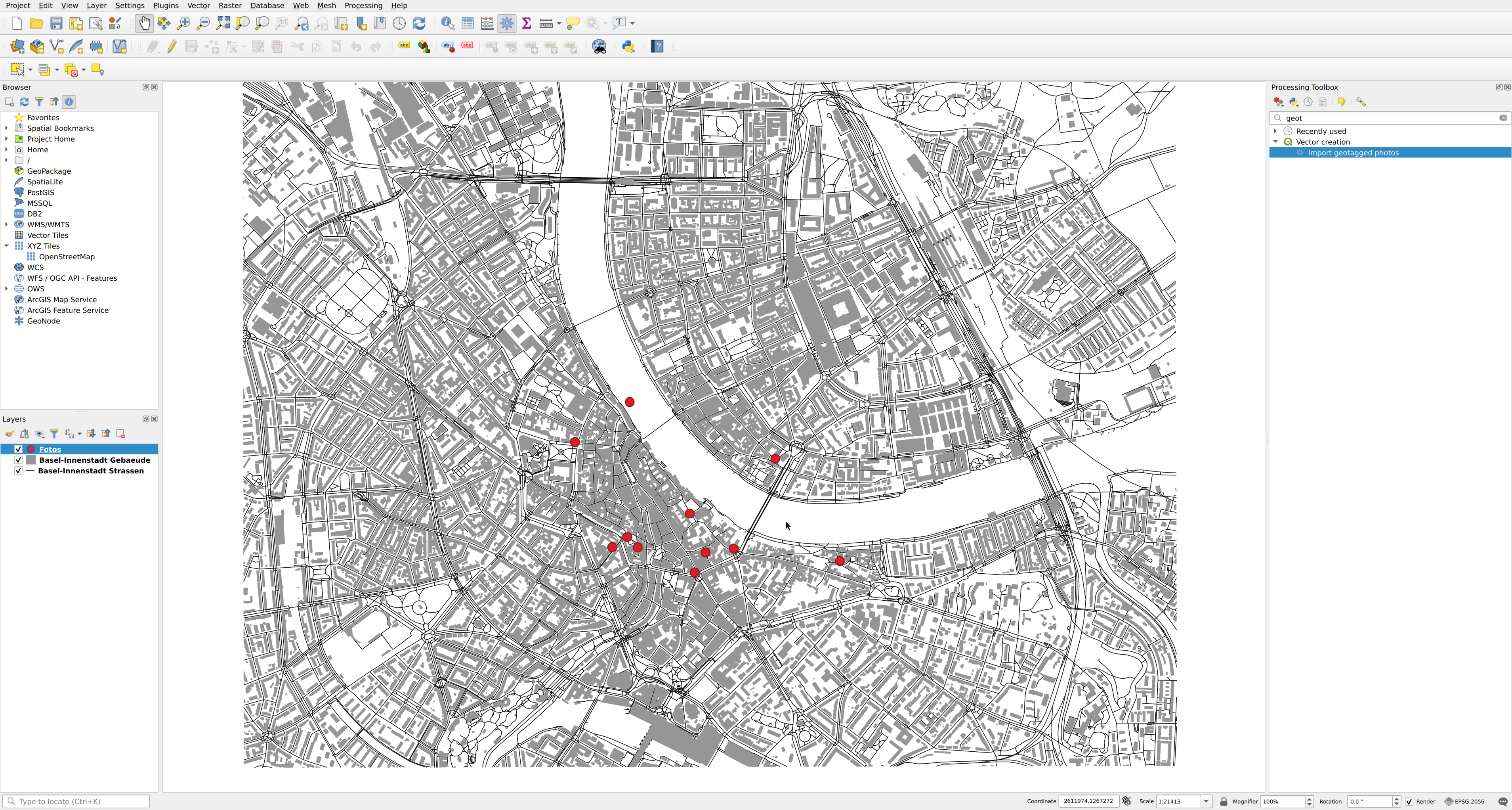
Now take a look at the layers in your project: The photo import has created a new layer. You will see several new points on the map. Each of these points stands for a photo taken at the respective location.
|
If you don’t see the photo points on the map well enough,
check the order of your layers and / or change the display settings of your photo layer in
|
Task 2: Show photos
You are probably wondering which photo is hidden behind which location.
With the identify features function  You can easily find this out in the toolbar:
Click on identify features and then on any location.
You can easily find this out in the toolbar:
Click on identify features and then on any location.
In the area Query results at the bottom right of the QGIS window, click on the button View feature form.
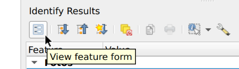
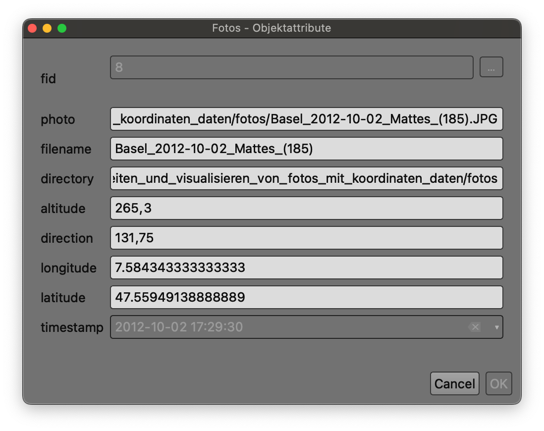
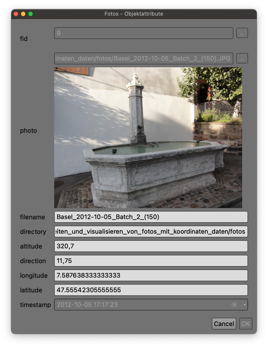
QGIS will now show you the object form for the selected photo location. This is already informative: In the photo field you can see which specific photo file is hidden behind the location. But wouldn’t it be much more convenient if the object form also displays this directly?
No problem! You can customize the presentation of the information it contains. To begin, first close the object form. Then open the properties of your photo layer by double-clicking on it in the layer list.
-
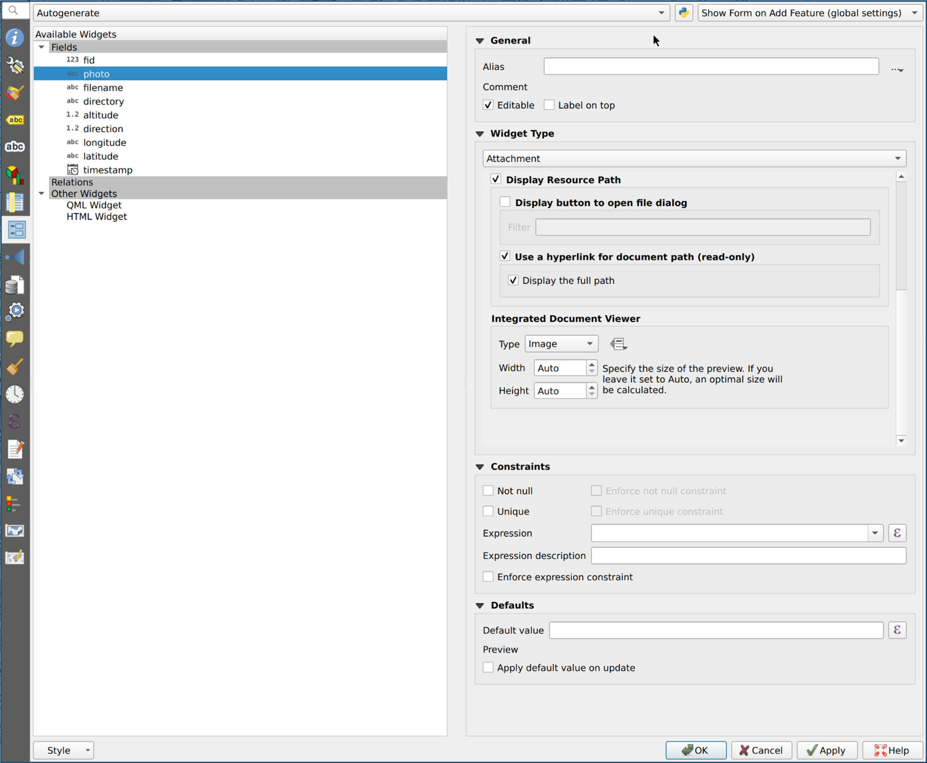
In the layer properties, click in the left list on Attributes form.
-
Select the photo entry in the "Available Widgets" list.
-
In Widget type, open the selection list and select the entry Attachment.
-
A little further down, a new section appears with the title Integrated document display. Open the selection list Type and select the image.
-
Once you have completed all settings, close the dialog by clicking on the OK button at the bottom right.
Now repeat the steps from the beginning of this task:
-
Click on the button Query objects
in the toolbar. -
Find a location on the map and click on it.
-
In the Query Results on the right, click Show object form.
Has anything changed compared to the first time?
|
Your adjustment in the object form also affects the attribute table.
In the toolbar at the top of your QGIS window Click on |
Exercise 3: Direction of view
In the previous exercises you learned how to import photos and then display them in QGIS. Take another look at the attribute form for one of the recording locations (see task 2) and take a closer look at the various fields. What kind of data do you recognize?
QGIS used the coordinates of the fields latitude and longitude to place the imported photos on your map. For the next step we are interested in the field direction
Imagine taking four photos: You take the first picture facing exactly north. For the next photo you turn in place and stand to the right, and photograph the scene to the east of you. You take the third photo in the south and the last in the west.
If you were to import these four photos into QGIS, they would all appear in exactly the same place. In this exercise you will learn how to use the direction field to reconstruct the direction the photographer is facing so that you can tell the individual photos apart.
-
Start in the processing tools, and type in the "search" field
 the term "wedge".
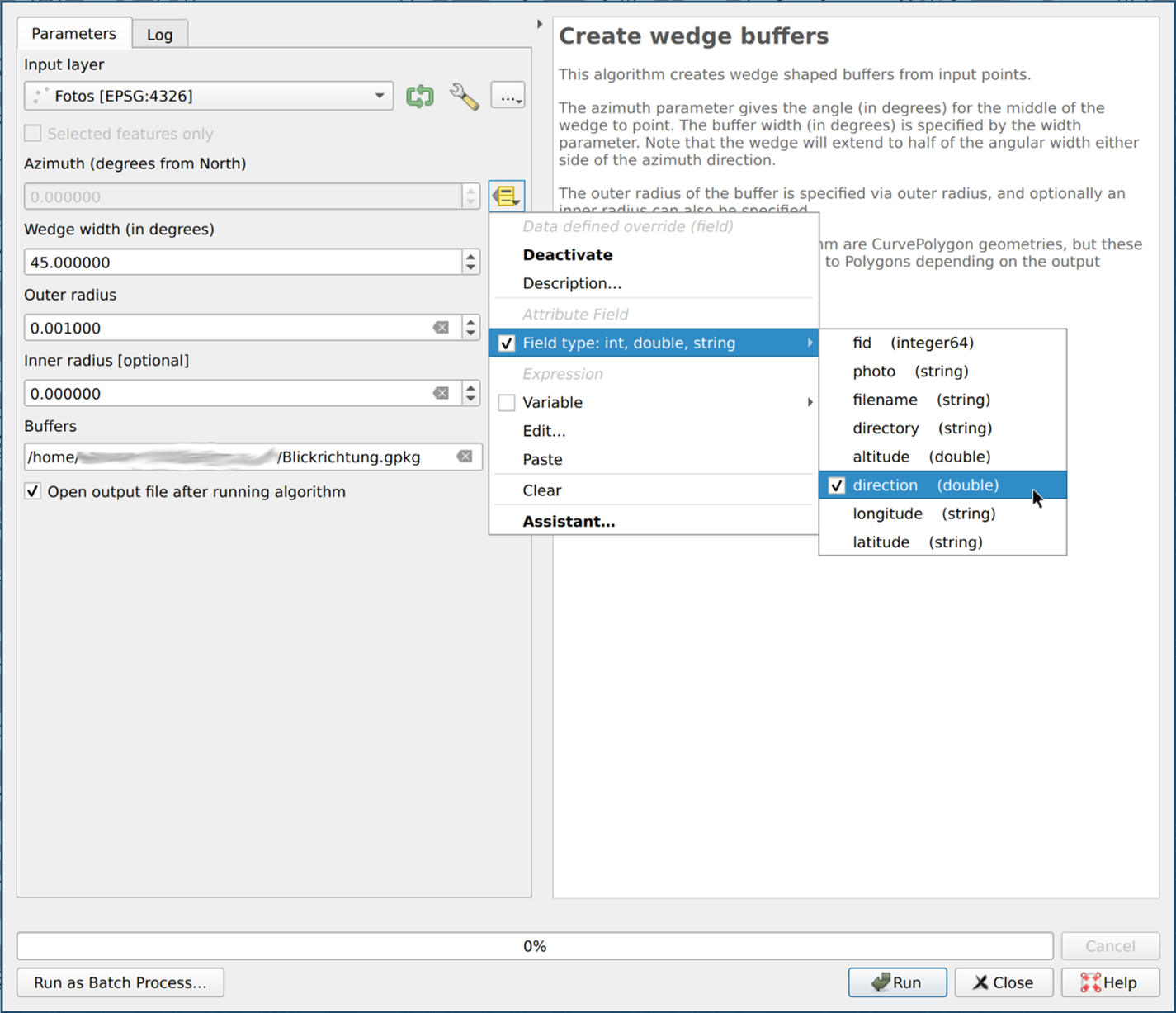
Open the tool Create wedge buffers in the search results with a double click.
the term "wedge".
Open the tool Create wedge buffers in the search results with a double click. -
If you haven’t already done so, select your photo layer from the Input layer selection list
-
Now link Azimuth (degrees to the north) with the direction field of the recording locations:
-
To do this, click on the button data-defined override
 to the right of the azimuth (degrees north) field
 -
select the entry field type: Integer, double, string
-
and confirm the link by clicking on direction (double) in the submenu.
-
-
Enter "0.001000" in the Outer radius field.
-
Next to the Buffer field, click on the button Browse
 and select any file from Save as …
in which the new layer with the viewing directions should be saved.
and select any file from Save as …
in which the new layer with the viewing directions should be saved. -
When you have finished with all the settings, click on Run in the lower right corner of the dialog and, after successful processing, on Close.
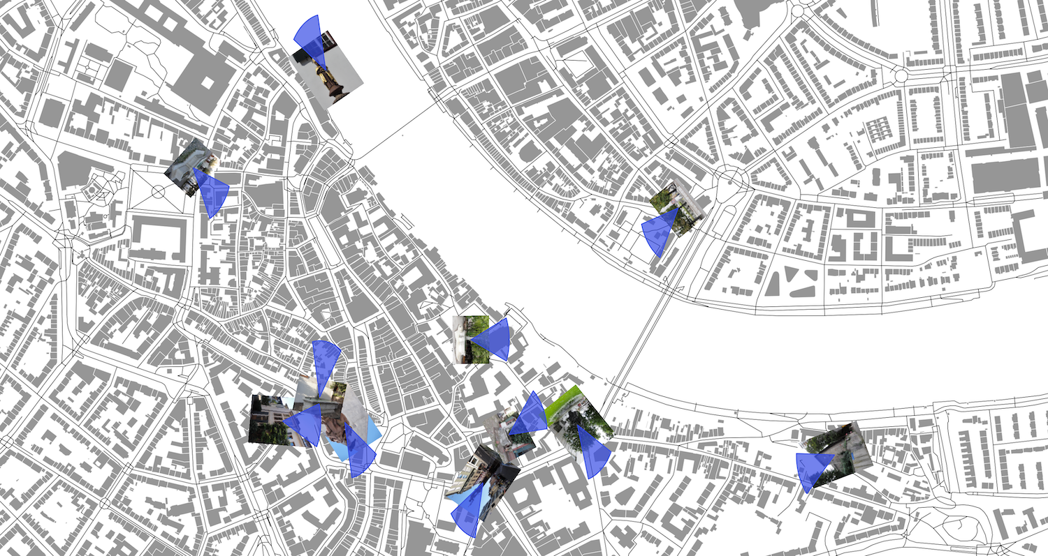
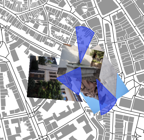
What happened? The Create wedge-shaped buffer has created a new layer, which has created a cone of vision for each recording location. The cone points exactly in the direction in which the photographer was looking while taking the picture.
You are almost certainly not satisfied with the way the cones of view are displayed, are you?
Double-click on the newly created layer in the layer list and
adjust the display in the sub-mune symbology ![]() according to your taste.
We decided on a blue border with a semi-transparent, blue filling.
according to your taste.
We decided on a blue border with a semi-transparent, blue filling.
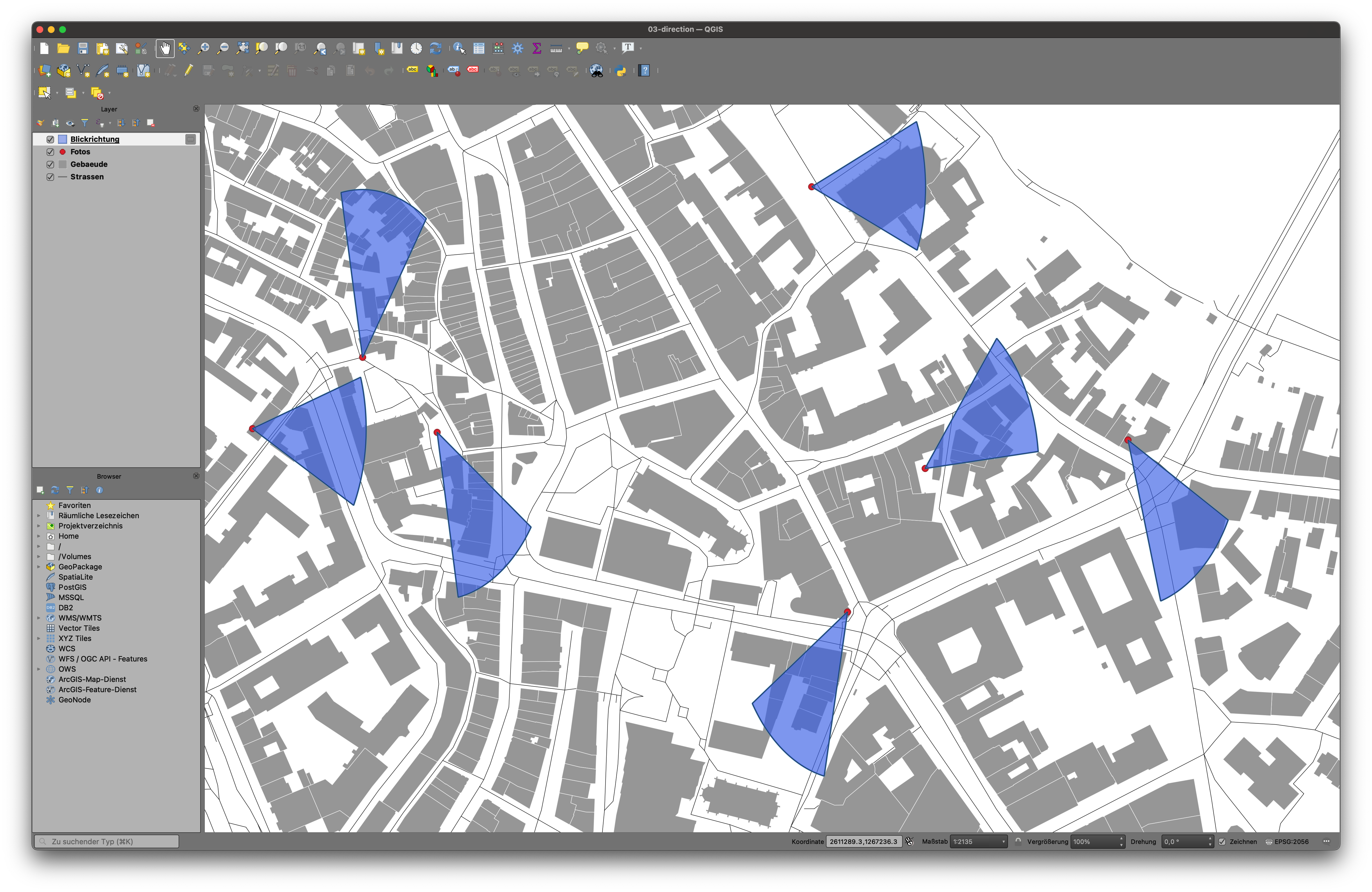
| You may be wondering why the cones of view appear to be a little "warped". This is related to the projection of the selected coordinate reference system (CRS). Further details can be found in the introductory worksheets from openschoolmaps.ch. |
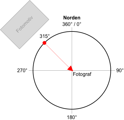
Digression for those interested: The direction value
In this exercise you used the direction field to show the photographer’s line of sight on the map.
This directional value follows the Degree Values on a Circle, which is oriented to the north. The photographer is always in the center of this circle.
If the photographer looks exactly to the north, this corresponds to a direction value of 0 degrees. If the photographer turns on the spot until he looks in the opposite direction, the direction assumes the value of 180 degrees.
Exercise 4: Photo miniatures
So far, your card shows a simple marker and visual cone for each photo. As a final step, you replace this simple marking with a miniature version of the stored photo.
Open the layer properties of your photo layer and select the sub-menu symbology image:aufbereiten-und-visualisieren-von-fotos-mit-koordinaten/aufgabe-3-symbolization.png [symbology, 20,20] to start.
-
Click on Simple marker in the upper list in the right half of the dialog.
-
Click on the selection list Symbol layer type, search for the entry raster image mark and select it with one click.
-
A large, empty field appears below the selection list:
-
Right-click on the Data-defined override
-
select the entry field type: string in the menu displayed
-
and link the field with the photo file by clicking on photo (string).
-
-
Repeat this process with the Rotation field. This time connect the field with direction (double), as you did in the previous exercise for the cone of vision.
-
Enter the number "30" in the Width field.
-
If you are satisfied with all the settings, click the OK button in the lower right corner of the dialog.
-
Raster image marker settings in the layer properties image::aufbereiten-und-visualisieren-von-fotos-mit-koordinaten/aufgabe-4-symbolisierung.png[. Raster image marker settings]
-
All the simple markings on your map have now disappeared and have been replaced with small photos. Did you notice that each photo is oriented like the cone of view you created in the previous task? Can you imagine why that is? (Tip: Which field, besides photo, have you also linked to the raster image marking?)
Bonus task: dynamic size for miniatures
View your map at different levels of magnification. Do you notice that the photos are always displayed in the same size? If you shrink the map more and more, the photos also begin to overlap.
Do you remember that a few steps ago, you entered a fixed width of "30" for the raster image marking? For this reason, the photo markings are always displayed in the same size, regardless of the magnification at which you are viewing the map. You can remedy this by not specifying the size of the photo markings, but making it dependent on the current zoom level.
To do this, open the layer settings of your photo layer again, select the sub-item
Symbology ![]() and click on the entry in the upper right area Raster image marking .
and click on the entry in the upper right area Raster image marking .
-
Right click Width field on the button Data-defined override
. -
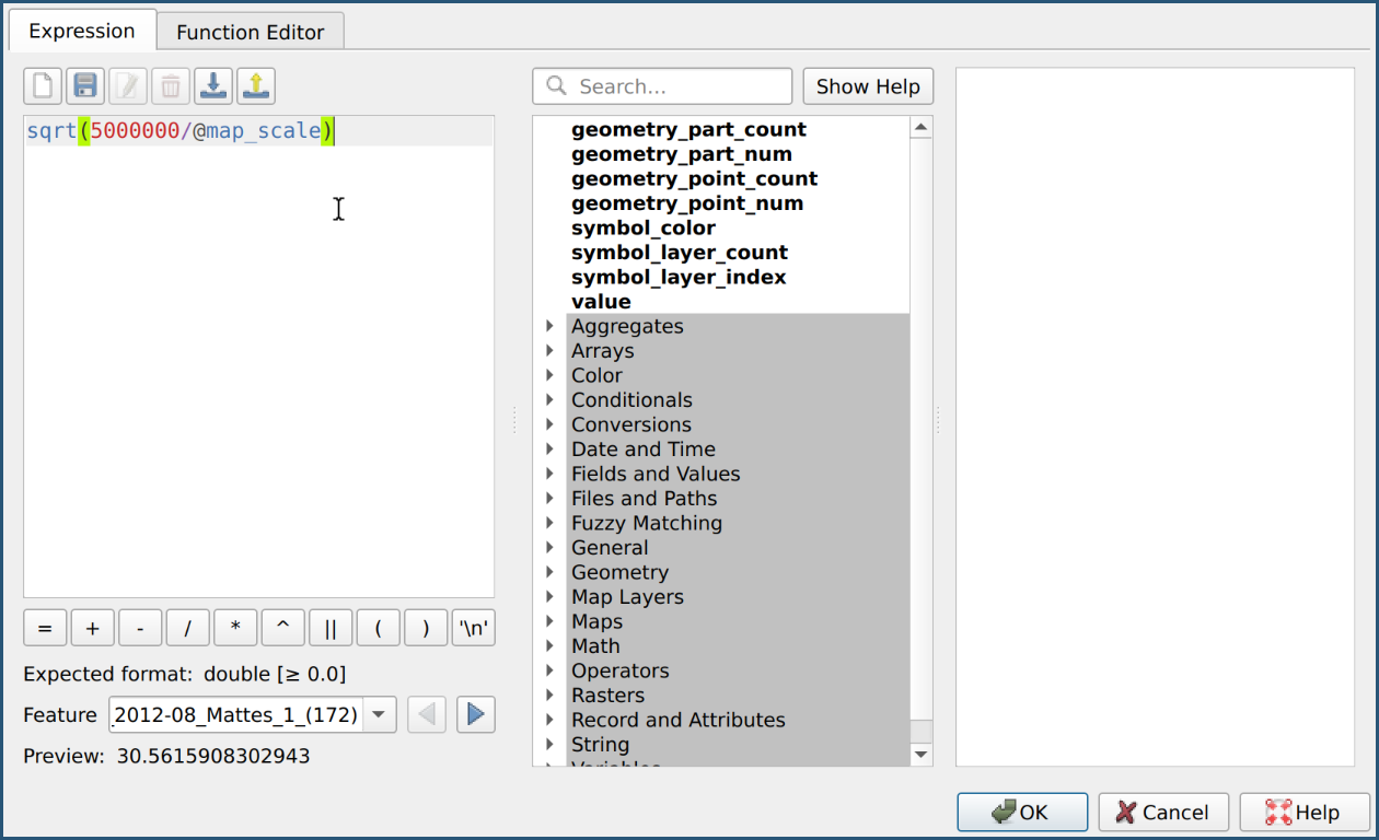
In the appeared menu, select the entry Edit …, to display the menu: Expression Editor [,]
-
Enter the following text in the left field:
sqrt (5000000 / @ map_scale) -
Close the expression editor and the layer settings each with a click on the btn: [OK] button at the bottom right
Change the magnification level of your map again. Do you notice a difference? Your photo markings no longer have a fixed size, but change depending on the current zoom level.
Completion
In the introduction to this worksheet you learned what metadata is for digital photos, what a geotag is and how geotags can be added to the metadata of photos or added manually.
In the exercises you gained your first experience with the photo import function of QGIS and learned how to display the locations and photos themselves as miniatures on a map.
In the bonus task, you also learned something about the directional value in the photo metadata. You then used this value to visualize the direction in which the photographer is looking on your map. This will give you an even better impression of the situation on site.
Outlook
Excursion for those interested: The expression editor
You can use the expression editor to display your layers,
make it even more flexible and dynamic.
In the bonus exercise you used the editor to link the variable @map_scale to the width of the photo miniature.
A variable is a placeholder for a value.
The variable @map_scale stands for the current zoom level of the map in QGIS.
Every time QGIS needs to calculate the width for a photo thumbnail,
it evaluates the mathematical expression sqrt (5000000 / @map_scale):
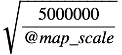
sqrt (5000000 / @map_scale) stands for the square root of 5,000,000 over @ map_scale.If you look at the map at a magnification of 25, QGIS calculates the width of a photo miniature using the following formula:
sqrt (5000000/25) stands for the square root of 5,000,000 over 25,which results in a width of 447.Try to change parts of the expression for the miniature width in the expression editor and observe the effects. The expression editor is a powerful tool in QGIS, a detailed description would go beyond the scope of this worksheet. If you would like to learn more about the possibilities of the expression editor, we recommend you take a look at the official manual of QGIS.
References
-
This worksheet is based on the chapter "Exercise 4 Mapping Photopoints" from the book "Discover QGIS: A Workbook for Classroom or Independent study "by Kurt Menke, ISBN 978-0998547763, published in 2020 at Locate Press LLC.
-
Source Figure 1: Manuel Alabor; made available for https://openschoolmaps.ch.
-
The photos used in the exercise part come from the following sources and are subject to the Creative Commons Attribution 2.0 Germany (CC BY 2.0 DE) License:
-
https://commons.wikimedia.org/wiki/File:Basel_2012-10-06_Batch_Part_5_(98).JPG
-
https://commons.wikimedia.org/wiki/File:Basel_2012-09-16_Batch_(15).JPG
-
https://commons.wikimedia.org/wiki/File:Basel_2012-10-02_Mattes_(185).JPG
-
https://commons.wikimedia.org/wiki/File:Basel_2012-09-16_Batch_(36).JPG
-
https://commons.wikimedia.org/wiki/File:Basel_2012-10-13_Batch_1_(62).JPG
-
https://commons.wikimedia.org/wiki/File:Basel_2012-09-28_Mattes_(149).JPG
-
https://commons.wikimedia.org/wiki/File:Basel_2012-08_Mattes_1_(233).JPG
-
https://commons.wikimedia.org/wiki/File:Basel_2012-08_Mattes_1_(172).JPG
-
https://commons.wikimedia.org/wiki/File:Basel_2012-09-16_Batch_(92).JPG
-
https://commons.wikimedia.org/wiki/File:Basel_2012-10-06_Batch_Part_5_(115).JPG
-
https://commons.wikimedia.org/wiki/File:Basel_2012-09-28_Mattes_(241).JPG
-
https://commons.wikimedia.org/wiki/File:Basel_2012-10-05_Batch_2_(150).JPG
-
-
The map material used was made using HOT Export Tool from OpenStreetMap exported on 11/21/2020.
.JPG)
.JPG)
.JPG)
.JPG)
.JPG)
.JPG)
.JPG)
.JPG)
.JPG)
.JPG)
.JPG)
.JPG)
Thanks
Many thanks go to Mr.Manuel Alabor - Student at the OST Campus Rapperswil. He designed this exercise.
Open questions? Feel free to contact OpenStreetMap Schweiz or Stefan Keller!
![]() Freely usable under CC0 1.0
Freely usable under CC0 1.0