A worksheet with exercises for self-learners and students.
| There’s a public repository on GitLab associated with this document. |
1. Overview
This worksheet is an introduction to OpenStreetMap (including Overpass API and the Overpass Turbo GUI) and more can be found at OpenSchoolMaps.
Learning Goals
This document is a compilation of solutions and tips for the following:
-
How to extract and geo-visualize OSM data on a map?
-
How to display OSM in an interactive map?
-
How to geocode your own data containing addresses and geonames?
-
How to do a spatial join with 3rd party open data?
Time Required
The time required to complete this worksheet is about 40 minutes including the initial setup, but this can vary depending on your previous knowledge and skills.
Prerequisites
Prerequisite for this solution is that the following software is installed (see bibliography and resources below):
-
Python 3,
-
Jupyter Notebook,
-
Some libraries (see
environment.ymlof Jupyter Notebook).
2. Introduction
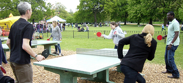
A Showcase - Outdoor Table Tennis Tables!
Let’s use outdoor table tennis tables or table tennis courts as a showcase from the story “Zurich is the hottest place in Switzerland to play ping-pong (according to OpenStreetMap of course 😉)”.
What is OpenStreetMap? – A Short Introduction
OpenStreetMap (OSM) is a free, editable map of the whole world, a crowdsourced project of open geospatial data. It’s the largest community in the geospatial domain, 2nd only to Wikimedia regarding community size, and 2nd to Google Maps regarding market share of base maps, Points-of-Interest (POI), etc..
It covers base maps, POI, routing and geocoding (building addresses).
The data structure consists of key-value pairs, called Tags, as attributes (“NoSQL Schema”), and it has a topological vector-geometry model based on Nodes, Ways plus Relations:
-
Node: osm_id, lat/lon coordinates, set of tags.
-
Way: osm_id, array of Node osm_ids (foreign keys), set of tags.
The OSM data structure is quite different from traditional Geographic Information Systems (GIS) (no layers) and from typical relational database models (no distinct attributes, like name, class). This means among other things:
-
It’s still possible to manage Point, Lines and Polygons (polygons are either closed ways or a relation referring to a set of ways).
-
Real world objects can be modelled either as Point, Line and Polygon.
An entity in OSM consists mostly of visually built parts - only rarely including a function. Details are added piecewise. There’s no strict conceptual modelling of an entity like in Software Engineering and in GIS services.
This means that an element like the following represents no single aspects
-
church: is a building, can be a historic place, can be a place of worship and can be many more
-
bath: can be a private swimming pool, a public bath, a park with bathing facilities, a water park, … See e.g. this Overpass query which tries to catch all bath objects in OSM:
[out:json];
area["name"="Schweiz/Suisse/Svizzera/Svizra"];
(
  nwr[sport=swimming][name](area);
  nwr[leisure=swimming_area][name];
  nwr[leisure=water_park];
  nwr[amenity=public_bath];
);
out center;
Extracting, processing and geo-visualizing OSM data on a map
-
Load OSM data (step 1),
-
Process and save it as a GeoJSON file (step 2)
-
Geovisualize the file as a static map with a base map.
Solution with ~50 lines of Python code
First find out what the tag (i.e. the key/value pair of table tennis tables) is: It’s “sport=table_tennis”. And let’s check this with Overpass-Turbo GUI with this link.
/*
Table Tennis Tables
*/
[out:json];
node["sport"="table_tennis"]({{bbox}});
out body; >; out skel qt;
This is a Python script solution with about 50 lines of Python code. We will use the same code in the next chapter using Jupyter.
import plotly.express as px
import geopandas as gpd
import matplotlib.pyplot as plt
from collections import namedtuple
from osm2geojson import overpass_call, json2geojson

# BBox with components ordered as expected by overpass.ql_query
Bbox = namedtuple("Bbox", ["south", "west", "north", "east"])
Tag = namedtuple("Tag", ["key", "values"])

def load_osm_from_overpass(bbox, tag, crs="epsg:4326") -> gpd.GeoDataFrame:
    geojson = load_osm_from_overpass_geojson(bbox, tag, crs)
    return gpd.GeoDataFrame.from_features(geojson, crs=crs)

def load_osm_from_overpass_geojson(bbox, tag, crs="epsg:4326"):
    values = None if "*" in tag.values else tag.values
    query = f"""
    [out:json];
    node["{tag.key}"="{values[0] if values else '*'}"]({bbox.south},{bbox.west},{bbox.north},{bbox.east});
    out body;
    >;
    out skel qt;
    """
    response = overpass_call(query)
    return json2geojson(response)

def plot_gdf_on_map(gdf, color="k", title=""):
    fig = px.scatter_mapbox(
        gdf,
        lat=gdf.geometry.y,
        lon=gdf.geometry.x,
        color_discrete_sequence=["fuchsia"],
        height=500,
        zoom=11,
    )
    fig.update_layout(title=title, mapbox_style="open-street-map")
    fig.update_layout(margin={"r": 0, "l": 0, "b": 0})
    return fig

def main():
    # Example: Table tennis tables in Zurich
    tag = Tag(key="sport", values=["table_tennis"])
    bbox_zurich = Bbox(west=8.471668, south=47.348834, east=8.600454, north=47.434379)
    table_tennis_gdf = load_osm_from_overpass(bbox_zurich, tag)
    gdf = table_tennis_gdf.to_crs(epsg=3857)
    gdf.geometry = gdf.geometry.centroid
    gdf = gdf.to_crs(epsg=4236)
    fig = plot_gdf_on_map(gdf, title="Zurich Table Tennis")
    # If no window appears, uncomment the following line
    # and open the standalone_map.html in your browser
    # fig.write_html("standalone_map.html")
    fig.show()

if __name__ == "__main__":
    main()
Listing 1: The Jupyter Notebook script in Python.
Task: Modify the script to display all drinking water fountains in Rapperswil-Jona. Find the appropriate tag and adjust the bounding box (Bbox) accordingly.
You can find the solution in the solutions.py file within the solutions directory.
| You can use bboxfinder or alternatively BBOX Webtool to get the coordinates of Rapperswil. |
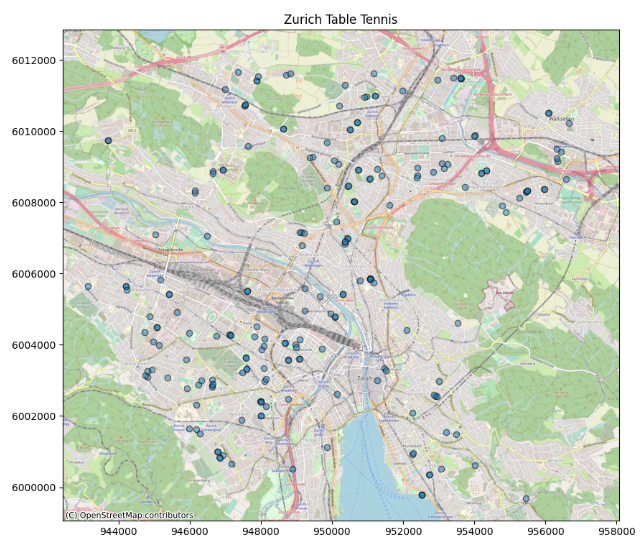
The result visualized with Matplotlib
Interactive map in a Jupyter Notebook
Python code can be used as above. You just have to call it directly instead of main().
Jupyter Notebooks with library Folium
There are many resources on the web for an introduction to Jupyter. So this is just a brief introduction: A Jupyter Notebook is a web-based interactive software environment with which Jupyter Notebook documents can be created. A Jupyter notebook document is a JSON file (with extension .ipynb). It contains a list of input and output cells, each of which can contain code, text and plots (i.e. maps).
| It’s very easy to execute a notebook document on the free web service MyBinder, for example. You can also host the notebooks yourself using Anaconda |
Publish map on the web
Next, we want to publish the map created in Jupyter Notebook on the web, without a backend, i.e. as generated HTML5 files (incl. Javascript and CSS). This can be done by using "export" with Folium: see solutions in the solutions directory.
The “magic 3 steps” of location analytics
The “magic 3 steps” of location analytics consist of the combination of your own data with foreign open data. This so-called “Geographic Data Enrichment” process (here’s a post) is possible, since location is “the universal foreign key”.
One of the crucial processes and services is the enhancement of your own data - which most probably contains a geoname or an address or such - using so-called geocoding, which is a quite a topic on its own.
Geocoding is the assignment of a coordinate given a postal address or a geoname.
So, given geonames or address data,
-
step one is to geocode your own data, which should contain an address or a geoname (i.e. adding a coordinate attribute), then
-
step two is to spatially join (i.e. combining) it with 3rd party geodata (like table tennis tables) using geospatial software (like PostGIS), then finally
-
step three, do the data analysis or geovisualization.
We’ll show this using PostgreSQL with the extension PostGIS and using the built-in language pl/pgsql plus Python.
| An easy alternative to geocoding - besides the approach with Python and PostgreSQL/PostGIS we’ll show here - would be using this online service from Localfocus.nl. For commercial geocoders see also “Help! I need a geocoder”. |
Step 1: Geocoding addresses and geonames
Let’s look at the core of a geocoding function in Python, which is wrapped as a PostgreSQL function in PL/pgSQL language.
|
In case
|
Add the missing parameters to get the coordinates of Vulkanstrasse 106, Zürich.
| You might want to take a look into the Nominatim-API. |
CREATE LANGUAGE plpythonu;

CREATE OR REPLACE FUNCTION geocode(address text)
RETURNS text AS $$
"""Returns WKT geometry which is EMPTY if address was not found.

Please respect the Nominatim free usage policy:
https://operations.osmfoundation.org/policies/nominatim/
"""

import requests
from time import sleep

base_url = 'https://nominatim.openstreetmap.org/search?'
params = {
    'q': address,
    'format': 'json',
    'limit': 1,
    'User-Agent': 'geocode hack (pls. replace)'
}
response = requests.get(base_url, params=params)
loc = response.json()
if len(loc) == 0:
    wkt = 'SRID=4326;POINT EMPTY'
else:
    wkt = f'SRID=4326;POINT({loc[0]['lon']} {loc[0]['lat']})'
sleep(1)  # Throttle, to avoid overloading Nominatim
return wkt
$$ LANGUAGE plpythonu VOLATILE COST 1000;

-- Test:
SELECT ST_AsGeoJSON(geocode('Vulkanstrasse 106, Zürich'));
Discussion:
-
This is just the code. It hasn’t yet run. We’ll do this within a single SQL query in step two below (BTW.: please respect the Nominatim free usage policy).
-
WKT -“Well Known Text” for encoding of geometries; example
POINT(47.36829, 8.54836). -
SRID=4326- Spatial Reference ID, an ID for the coordinate reference system WGS84, known for lat/lon coordinates. -
Please replace
geocode hackfromUser-Agentwith a user agent name specific to you. Otherwise you risk being banned from the Nominatim service.
Step 2: Joining spatially
Now - given we have the geocoding function in place - we do a spatial join. This means combining our data - like three addresses - with 3rd party geodata - like table tennis tables - using a geospatial software (like PostGIS). We will use a dataset of OSM Switzerland imported into a PostgreSQL/PostGIS instance using the osm2pgsql bulk loader tool.
And that’s what we’d like to analyse: Give me a list of the five closest table tennis tables with related ‘customers’. Output: customer_id, distance, osm_id + osm_type (Node, Way, Relation), geometry.:
-
1: Vulkanstrasse 106, Zürich
-
2: Bellevue, 8001 Zürich
-
3: Weihnachtsmann
WITH my_customers_tmp(id, address, geom) AS (
  SELECT id, address, ST_Transform(ST_MakeValid(GeomFromEWKT(geocode(address))),3857) AS geom
  FROM (values
   (1,'Vulkanstrasse 106, Zürich'),
   (2,'Bellevue, 8001 Zürich'),
   (3,'Weihnachtsmann')
  ) address(id,address)
),
poi_tmp AS (
  SELECT
        osm_id,
        gtype,
        -- POI address would need to reverse_geocode!
        tags,
        way AS geom FROM osm_poi
  WHERE tags->'sport' IN ('table_tennis')
)
SELECT
  my_customers_tmp.id as customer_id,
  ST_Distance(my_customers_tmp.geom, poi_tmp.geom)::integer AS distance,
  poi_tmp.osm_id,
  poi_tmp.gtype,
  ST_Transform(poi_tmp.geom,4326) AS geom
FROM my_customers_tmp, poi_tmp
ORDER BY my_customers_tmp.geom <-> poi_tmp.geom
LIMIT 5;
Listing 3: SQL query of the geocode hack with Nominatim API in Python and PostgreSQL/PostGIS.
Discussion:
-
This is a modern SQL query using a Common Table Expression (a
WITHstatement). It puts the geocoding result in a temporary tablemy_customers_tmp. -
The second temporary table
poi_tmpstores the table tennis tables and queries from base tableosm_poi, which is a view on osm_point and osm_polygon from an OSM database containing Swiss data (osm_poithus is similar to the "nwr and center" in the Overpass query from before). -
The note “POI address would need to reverse_geocode!” tries to indicate that you would probably want to get addresses for the POI - here: table tennis tables - found.
Step 3: Doing the data analysis…
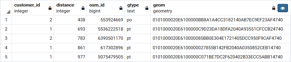
This is the result of the spatial SQL query above:
Discussion:
-
Customer 2 from Bellevue is closest to a table tennis table, distance 438 meters.
-
Customer 1 from Vulkanstrasse is second, distance 693 m.
-
Customer 3, the Weihnachtsmann 🎅 isn’t appearing in the data output of the query - the geocoder did not find an address for this place.
3. Conclusion and Outlook
We’ve mainly used the following software: The Overpass API service and the PostgreSQL/PostGIS tool (see fig. 4).
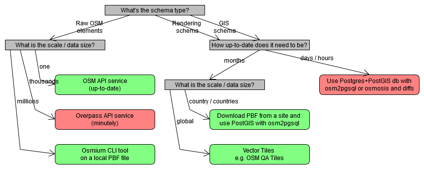
The advantages of the Overpass API service are that it’s a service and that it contains up-to-date data. The drawbacks of the service are that the result data can’t contain more than a few thousand features and that the query language is weird and limited.
The advantage of PostgreSQL/PostGIS is the spatial SQL query interface (see e.g. these tips and tricks). The drawbacks of this tool are the installation time and the local resources needed - plus the issue that PostGIS queries (and osm2pgsql bulk loader) can’t yet be parallelized - though they’re still fast enough for many applications if used properly with the right indexes and operators (e.g. KNN <→).
Beside the special web service Overpass API called from Python, there are other approaches like SQL together with pgRouting, which is another PostgreSQL extension like PostGIS.
There is also an interesting university course which includes “Download and visualize OpenStreetMap data with OSMnx”. OSMnx is quite useful and the course covers many GIS topics, from vector overlay and network analysis to raster data analysis.
In the end, data is everything. So the question remains: How to discover more open geodata? There is no simple answer to this question and it requires much experience. See e.g. opendata.swiss or “Freie Geodaten” for a start.
Last but not least, the learning portal OpenSchoolMaps should be mentioned again, which is being periodically updated with new learning materials.
4. Bibliography and Resources
Installing Jupyter software locally (Windows):
Jupyter Notebooks / How-to’s:
-
Different open source tools for geospatial data visualization in Jupyter Notebooks (Python): https://medium.com/@bartomolina/geospatial-data-visualization-in-jupyter-notebooks-ffa79e4ba7f8
-
OSMNx: “Download and visualize OpenStreetMap data with OSMnx” (Python)
-
“A Guide: Turning OpenStreetMap Location Data into ML Features - How to pull shops, restaurants, public transport modes and other local amenities into your ML models.” by Daniel L J Thomas, Sep 17 2020. https://towardsdatascience.com/a-guide-turning-openstreetmap-location-data-into-ml-features-e687b66db210 (Note: includes OSMnx, Overpass, K-D Tree to calculate distances)
Software libraries and frameworks for OSM and Python:
-
Python Lib “OSMnx” (Line Network, POI): https://osmnx.readthedocs.io/en/stable/osmnx.html#module-osmnx.pois and https://automating-gis-processes.github.io/site/notebooks/L6/retrieve_osm_data.html
-
Other Python Libs: “Overpass API python wrapper” by mvexel: https://github.com/mvexel/overpass-api-python-wrapper . OverPy: https://github.com/DinoTools/python-overpy .
-
“Awesome OpenStreetMap” - A curated list of ‘everything’ about OpenStreetMap (not yet as complete as one would wish): https://github.com/osmlab/awesome-openstreetmap#python
Overpass API and GUI:
-
Overpass API: https://towardsdatascience.com/loading-data-from-openstreetmap-with-python-and-the-overpass-api-513882a27fd0
-
How to use Overpass: https://gis.stackexchange.com/questions/203300/how-to-download-all-osm-data-within-a-boundingbox-with-overpass
-
Typical Overpass Query:
[out:json];
area["ISO3166-2"="CH-ZH"];
(
  nwr[sport="table_tennis"](area);
  nwr[leisure="table_tennis_table"];
);
out center;
Any more questions? Please contact Stefan Keller (stefan.keller@ost.ch)!
![]() Freely usable under CC0 1.0: http://creativecommons.org/publicdomain/zero/1.0/
Freely usable under CC0 1.0: http://creativecommons.org/publicdomain/zero/1.0/